Michele Coscia

Networks are cool because they’re a relatively simple model that allows you to understand complex systems. The problem is that they’re too cool: sometimes they make you want to do network analysis on something that isn’t really a network. For instance, consider Netflix. Here you have people watching movies. You want to know which movies are similar to each other so that you can suggest them to similar users. On the wings of Maslow’s Law — when you’re holding a hammer everything starts looking like a nail –, the network scientist would want to build a movie-movie network.

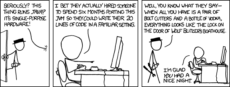
Of course XKCD has something about this.

The problem is that there are many different ways to make a movie-movie network from Netflix data. Each of these different ways will alter the shape of your network in dramatic ways, which will affect the results you’re going to get once you use it for your aims. With Luca Rossi, I started exploring this space. This resulted in the paper “The Impact of Projection and Backboning on Network Topologies“, which I will present next week at the ASONAM conference.

In the paper we take some real-world data and we apply all possible combinations of network building techniques on it. We systematically explore the key topological properties of the resulting networks, and see that they dramatically change depending on which strategy you picked. Meaning that you’re going to get completely different results from the same analysis later on.

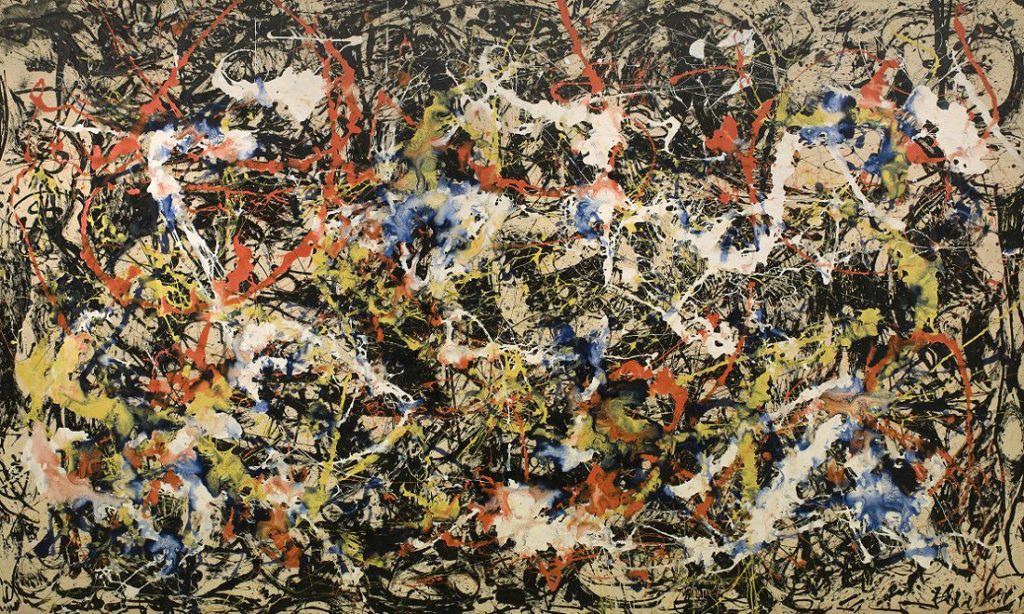
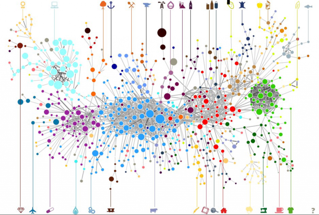
Good network analysis is like good art: if you gaze long at the hairball, the hairball will gaze back at you. Image property of the Albright-Knox Art Gallery, Buffalo, NY.

The first thing we need to understand is that, to get to the movie-movie network, we need to perform two major steps. Each movie is a vector, containing information about each user. It could simply be a one if the user watched the movie, or a zero if they didn’t. Thus first we need to apply a similarity measure quantifying how similar two movies are to each other (what I call “projection”). Then we’ll realize that all we got is a hairball. Every movie has a non-zero similarity with any other movie. After all, there are millions of users, but just a handful of movies, so the probability that any two movies were watched by at least one user is pretty high. So you need to filter out your movie-movie similarity, otherwise your resulting network will be too dense.

Comparing two vectors is the oldest profession in the world, assuming your world is completely made up of linear algebra — mine, sadly, is. Thus you can pick and choose dozens of similarity metrics — Euclidean, cosine, I have a soft spot for the Mahalanobis distance myself. However, you’d be better served by the measures that were developed with complex networks in mind. You see, the binary movie-user vectors will have typical broad degree distributions: some movies are very popular — everybody watches them –, some people like me are pathological movie buffs and will watch everything — my watchlist has ~6,500 entries. Thus for this paper we focus on a few of those “bipartite projection” techniques: hyperbolic, resource allocation (ProbS), and my beloved YCN method.

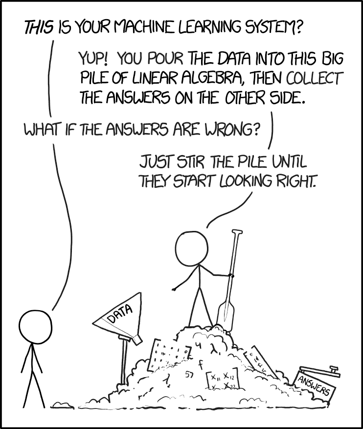
Since I already jumped on the XKCD wagon, I see no harm in continuing down this path…

Then, to filter out connections, you have to have an idea of what’s a “strong, significant” connection and what isn’t. If you’re naive and just think that you should only keep connections with higher weights (what I call “naive thresholding”), boy do I have news for you. Also in this case, we’re going to consider a couple of ways to filter out noisy connections: the disparity filter and my noise corrected backbone.

Ok, the stage is set. If you were paying attention, you’ll figure out what’s coming next: a total mess.

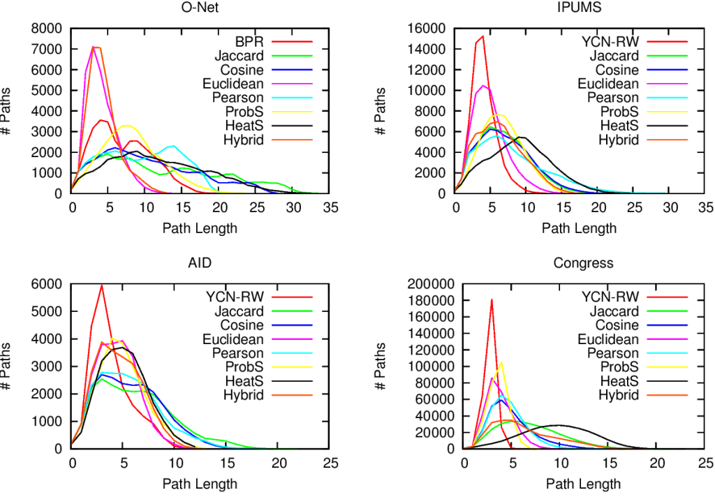
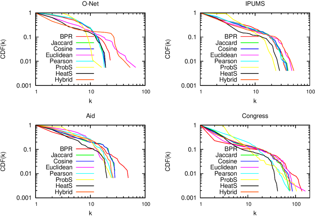
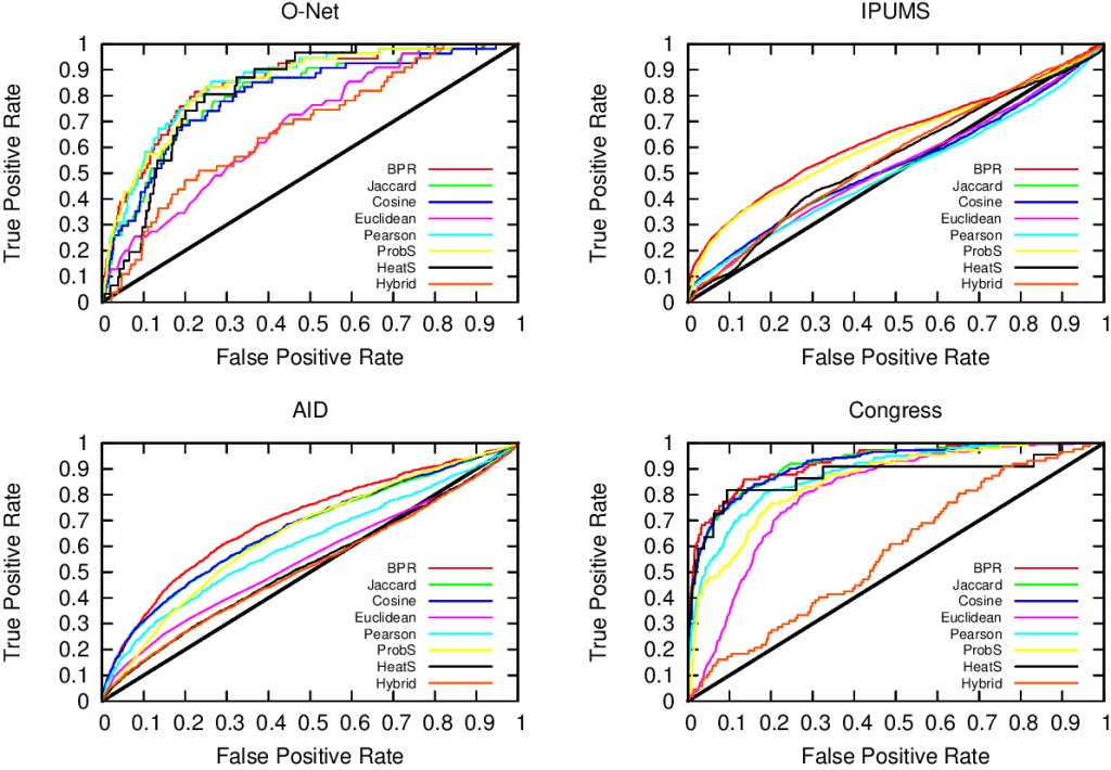
Above (click to enlarge) you see the filtering techniques — top to bottom: naive threshold, disparity filter, noise corrected –, for each projection — line color –, on different network properties. From left to right we see: how many nodes survive the filter step, how much clustered the network is, and how well separated its communities are. The threshold levels (x-axis) attempt to preserve a comparable number of edges for each technique combination.

Yeah, it doesn’t look good. Look at the middle column: there are some versions of this network with perfect clustering, meaning that every common neighbor of a movie is connected to every other; while networks have a transitivity of zero; with almost every possible other values in between. The same holds for modularity, which can span from ~0.2 to practically 1. So there’s no way of saying whether these are properties of the system or just properties of the cleaning procedures you used. Keep in mind that the original data is the same. We could conclude anything by stirring our pile of linear algebra. Want to argue that the movie space doesn’t cluster? Project with YCN and filter with noise corrected method. Want to find strong communities instead? No biggie: project with resource allocation and do a simple threshold of the result.

Famous network scientist and two-time “world’s best mustache” winner Nietzsche once said: “He who fights with hairballs should look to it that he himself does not become a hairball.”

I wish I had a wise message to wrap up this blog post. Something about how to choose the best projection-filtering pair best fitting a specific analysis — one that you cannot tune to obtain the results you want. However, that will have to wait for further research. For now, I just want you to grow suspicious about specific results you see out there from networks that really aren’t network. If your nodes aren’t really connecting directly — like physical connections would do, for instance between neurons –, pretending they do so might lead you down a catastrophic over-confident path.

Continue Reading

When reporting on economics, news outlets very often refer to what happens to the GDP. How is policy X going to affect our GDP? Is the national debt too high compared to GDP? How does my GDP compare to yours? The concept lurking behind those three letters is the Gross Domestic Product, the measure of the gross value added by all domestic producers in a country. In principle, the idea of using GDP to take the pulse of an economy isn’t bad: we count how much we can produce, and this is more or less how well we are doing. In practice, today I am jumping on the huge bandwagon of people who despise GDP for its meaningless, oversimplified and frankly suspicious nature. I will talk about a paper in which my co-authors and I propose to use a different measure to evaluate a country’s prosperity. The title is “Going Beyond GDP to Nowcast Well-Being Using Retail Market Data“, my co-authors are Riccardo Guidotti, Dino Pedreschi and Diego Pennacchioli, and the paper will be presented at the Winter edition of the Network Science Conference.

GDP is gross for several reasons. What Simon Kuznets said resonates strongly with me, as already in the 30s he was talking like a complexity scientist:

The valuable capacity of the human mind to simplify a complex situation in a compact characterization becomes dangerous when not controlled in terms of definitely stated criteria. With quantitative measurements especially, the definiteness of the result suggests, often misleadingly, a precision and simplicity in the outlines of the object measured. Measurements of national income are subject to this type of illusion and resulting abuse, especially since they deal with matters that are the center of conflict of opposing social groups where the effectiveness of an argument is often contingent upon oversimplification.

In short, GDP is an oversimplification, and as such it cannot capture something as complex as an economy, or the multifaceted needs of a society. In our paper, we focus on some of its specific aspects. Income inequality skews the richness distribution, so that GDP doesn’t describe how the majority of the population is doing. But more importantly, it is not possible to quantify well-being just with the number of dollars in someone’s pocket: she might have dreams, aspirations and sophisticated needs that bear little to no correlation with the status of her wallet. And even if GDP was a good measure, it’s very hard to calculate: it takes months to estimate it reliably. Nowcasting it would be great.

And so we tried to hack our way out of GDP. The measure we decided to use is the one of customer sophistication, that I presented several times in the past. In practice, the measure is a summary of the connectivity of a node in a bipartite network*. The bipartite network connects customers to the products they buy. The more variegated the set of products a customer buys, the more complex she is. Our idea was to create an aggregated version at the network level, and to see if this version was telling us something insightful. We could make a direct correlation with the national GDP of Italy, because the data we used to calculate it comes from around a half million customers from several Italian regions, which are representative of the country as a whole.

The argument we made goes as follows. GDP stinks, but it is not 100% bad, otherwise nobody would use it. Our sophistication is better, because it is connected to the average degree with which a person can satisfy her needs**. Income inequality does not affect it either, at least not in trivial ways as it does it with GDP. Therefore, if sophistication correlates with GDP it is a good measure of well-being: it captures part of GDP and adds something to it. Finally, if the correlation happens with some anticipated temporal shift it is even better, because GDP pundits can just use it as instantaneous nowcasting of GDP.

We were pleased when our expectations met reality. We tested several versions of the measure at several temporal shifts — both anticipating and following the GDP estimate released by the Italian National Statistic Institute (ISTAT). When we applied the statistical correction to control for the multiple hypothesis testing, the only surviving significant and robust estimate was our customer sophistication measure calculated with a temporal shift of -2, i.e. two quarters before the corresponding GDP estimate was released. Before popping our champagne bottles, let me write an open letter to the elephant in the room.

As you see from the above chart, there are some wild seasonal fluctuations. This is rather obvious, but controlling for them is not easy. There is a standard approach — the X-13-Arima method — which is more complicated than simply averaging out the fluctuations. It takes into account a parameter tuning procedure including information we simply do not have for our measure, besides requiring observation windows longer than what we have (2007-2014). It is well possible that our result could disappear. It is also possible that the way we calculated our sophistication index makes no sense economically: I am not an economist and I do not pretend for a moment that I can tell them how to do their job.

What we humbly report is a blip on the radar. It is that kind of thing that makes you think “Uh, that’s interesting, I wonder what it means”. I would like someone with a more solid skill set in economics to take a look at this sophistication measure and to do a proper stress-test with it. I’m completely fine with her coming back to tell me I’m a moron. But that’s the risk of doing research and to try out new things. I just think that it would be a waste not to give this promising insight a chance to shine.

* Even if hereafter I talk only about the final measure, it is important to remark that it is by no means a complete substitute of the analysis of the bipartite network. Meaning that I’m not simply advocating to substitute a number (GDP) for another (sophistication), rather to replace GDP with a fully-blown network analysis.

** Note that this is a revealed measure of sophistication as inferred by the products actually bought and postulating that each product satisfies one or a part of a “need”. If you feel that the quality of your life depends on you being able to bathe in the milk of a virgin unicorn, the measure will not take into account the misery of this tacit disappointment. Such are the perils of data mining.

Continue Reading

Complex networks can come in different flavors. As you know if you follow this blog, my signature dish is multilayer/multidimensional networks: networks with multiple edge types. One of the most popular types is bipartite networks. In bipartite networks, you have two types of nodes. For example, you can connect users of Netflix to the movies they like. As you can see from this example, in bipartite networks we allow only edges going from one type of nodes to the other. Users connect to movies, but not to other users, and movies can’t like other movies (movies are notoriously mean to each other).

Many things (arguably almost everything) can be represented as a bipartite network. An occupation can be connected to the skills and/or tasks it requires, an aid organization can be connected to the countries and/or the topics into which it is interested, a politician is connected to the bills she sponsored. Any object has attributes. And so it can be represented as an object-attribute bipartite network. However, most of the times you just want to know how similar two nodes of the same type are. For example, given a movie you like, you want to know a similar movie you might like too. This is called link prediction and there are two ways to do this. You could focus on predicting a new user-movie connection, or focus instead on projecting the bipartite network to discover the previously unknown movie-movie connections. The latter is the path I chose, and the result is called “Network Map”.

It is clearly the wrong choice, as the real money lies in tackling the former challenge. But if I wanted to get rich I wouldn’t have chosen a life in academia anyway. The network map, in fact, has several advantages over just predicting the bipartite connections. By creating a network map you can have a systemic view of the similarities between entities. The Product Space, the Diseasome, my work on international aid. These are all examples of network maps, where we go from a bipartite network to a unipartite network that is much easier to understand for humans and to analyze for computers.

Creating a network map, meaning going from a user-movie bipartite network to a movie-movie unipartite network, is conceptually easy. After all, we are basically dealing with objects with attributes. You just calculate a similarity between these attributes and you are done. There are many similarities you can use: Jaccard, Pearson, Cosine, Euclidean distances… the possibilities are endless. So, are we good? Not quite. In a paper that was recently accepted in PLoS One, Muhammed Yildirim and I showed that real world networks have properties that make the general application of any of these measures quite troublesome.

For example, bipartite networks have power-law degree distributions. That means that a handful of attributes are very popular. It also means that most objects have very few attributes. You put the two together and, with almost 100% probability, the many objects with few attributes will have the most popular attributes. This causes a great deal of problems. Most statistical techniques aren’t ready for this scenario. Thus they tend to clutter the network map, because they think that everything is similar to everything else. The resulting network maps are quite useless, made of poorly connected dense areas and lacking properties of real world networks, such as power-law degree distributions and short average path length, as shown in these plots:

Of course sometimes some measure gets it right. But if you look closely at the pictures above, the only method that consistently give the shortest paths (above, when the peak is on the left we are good) and the broadest degree distributions (below, the rightmost line at the end in the lower-right part of the plot is the best one) is the red line of “BPR”. BPR stands for “Bipartite Projection via Random-walks” and it happens to be the methodology that Muhammed and I invented. BPR is cool not only because its network maps are pretty. It is also achieving higher scores when using the network maps to predict the similarity between objects using ground truth, meaning that it gives the results we expect when we actually already know the answers, that are made artificially invisible to test the methodology. Here we have the ROC plots, where the highest line is the winner:

So what makes BPR so special? It all comes down to the way you discount the popular attributes. BPR does it in a “network intelligent” way. We unleash countless random walkers on the bipartite network. A random walker is just a process that starts from a random object of the network and then it jumps from it to one of its attributes. The target attribute is chosen at random. And then the walker jumps back to an object possessing that attribute, again choosing it at random. And then we go on. At some point, we start from scratch with a new random walk. We note down how many times two objects end up in the same random walk and that’s our similarity measure. Why does it work? Because when the walker jumps back from a very popular attribute, it could essentially go to any object of the network. This simple fact makes the contribution of the very popular attributes quite low.

BPR is just the latest proof that random walks are one of the most powerful tools in network analysis. They solve node ranking, community discovery, link prediction and now also network mapping. Sometimes I think that all of network science is founded on just one algorithm, and that’s random walks. As a final note, I point out that you can create your own network maps using BPR. I put the code online (the page still bears the old algorithm’s name, YCN). That’s because I am a generous coder.

Continue Reading