25 March 2020 ~ 0 Comments

How Quickly is COVID Really Spreading?

I don’t need to introduce to you what the corona virus is: COVID-19 has had a tremendous impact on everyone’s life in the past weeks and months. All of a sudden, our social media feeds have been invaded with new terminology: social distancing, R0, infection rate, exponential growth. Overnight, we turned ourselves into avid consumers of epidemics literature. We learned what the key to prevent the infection from becoming a larger problem is: slow the bugger down. That is why knowing how fast corona is actually moving is such a crucial piece of information. You have seen the pictures many times, they look something like this:
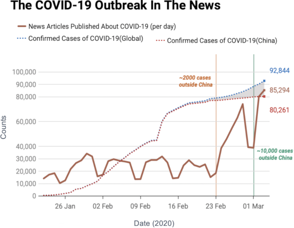
Image courtesy of my data science students: Astrid Machholm, Jacob Kristoffer Hessels, Marie-Louise Tommerup, Simon Breum, Zainab Ali Shaker Khudoir. If anything, it warms my heart knowing that, even during a pandemic, many journalists take their weekends off 🙂

What you’re seeing is the evolution in number of infected people — and how much non-infected people like me blabber about them online. Epidemiologists try to estimate the speed of infection by fitting the real data you see on an SI model. In it, people turn from Susceptible to Infected at a certain rate. These models are usually precise at estimating the number of infected over time, but they lack a key component: they assume that each individual is interchangeable and that anyone has a chance to be infected by anyone in their close proximity. In other words, they ignore the fact that we are embedded in a social network: some people are more central than others, and some have more friends than others.

To properly estimate how fast a disease moves, you need to take the network into account. And this is the focus of a paper of mine: “Generalized Euclidean Measure to Estimate Network Distances“. The paper has been accepted for publication at the 2020 ICWSM conference. The idea of the paper is to create a new measure that estimates the distance between the state of the disease at two moments in time, taking the underlying network topology into account.
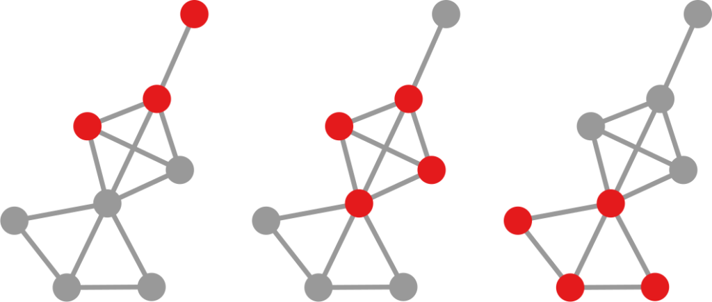
The question here is deceptively simple. Suppose you have a set of infected individuals. In the picture above, they are the nodes in red in the leftmost social network. After a while, some people recover, while others catch the disease. You might end up with the set of infected from the network in the middle, or the one in the right. In which case did the disease spread more quickly?

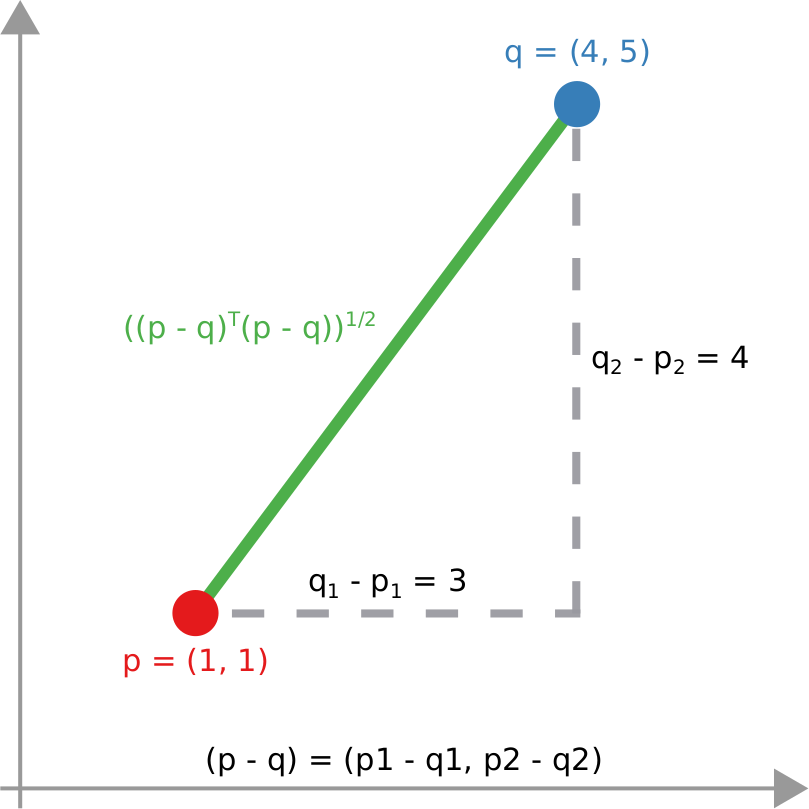
We have a clear intuitive answer: the rightmost network experienced a faster spread, because the infected nodes are farther from the original ones. We need to find a measure that matches this intuition. How do we normally estimate distances in the real world? We use a ruler: we draw a straight line between two points and we measure how long that line is. This is the Euclidean distance. Mathematically, that means representing the two points as vectors of coordinates (p and q), calculating their difference, and then using Pythagoras’ theorem to calculate the length of the straight line between them:

We cannot apply this directly to our network problem. This is because, for silly Euclid, every dimension has the same importance in estimating the distance between points. However, in our case, the points are the states of the disease. They do not live on the plane of Euclidean geometry, but on a network. Some moves in this network space are short and easy: moving between two connected nodes. But other moves are long and hard: between two nodes that are far apart. In other words, nodes that are connected to each other contribute less than unconnected nodes to the distance. The simplest example I can make is:

In the figure, each vector — for instance (1,0,0) — is the representation of the state of the disease of the graph beneath it: the entries equal to one identify the currently infected node. Clearly, the infection closer to the left graph is the middle one, not the right one. However, the Euclidean distance between the three vectors is the same: the square root of two. So how do we fix this problem? There is a distance measure that allows you to weigh dimensions differently. It is my favorite distance metric (yes, I am the kind of person who has a favorite distance metric): the Mahalanobis distance. Mahalanobis simply says that correlated variables should count less in estimating the distance: taller people tend to be heavier — because there’s more person to weigh — so we shouldn’t be surprised if someone taller than me is also heavier. But, if they weigh less, we would find it remarkable.

Now we’re just left with the problem of figuring out how to estimate, mathematically, what “correlated” means in a network. The paper has the full details. For here, suffice to say we augment Pythagoras’ theorem with the pseudoinverted graph Laplacian — a sentence I’m writing only to pretend I’m smart (it’s actually not sophisticated at all, and a super easy thing to calculate). The reason we use the graph Laplacian is because it is a standard instrument to estimate how fast things spread in a network.
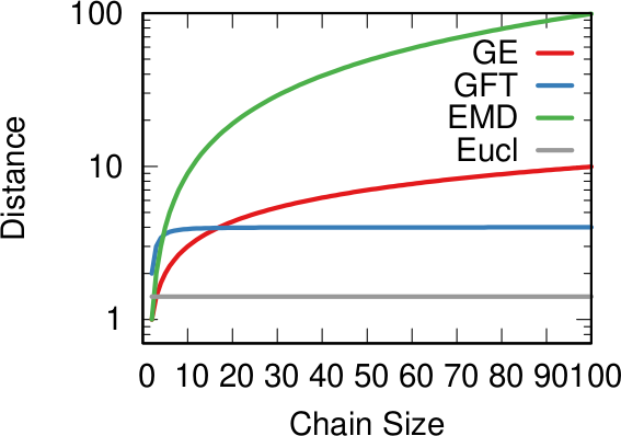
In the paper I run a bunch of tests to show that this measure matches our intuition. For instance, as shown above, if we have infected people at the endpoints of a chain graph, the longer the chain (x axis) the higher the estimated distance should be (y axis). GE (= Generalized Euclidean, in red) is my measure, and it behaves as it should: a constantly growing function (the actual values don’t really matter as long as they constantly grow as we move left to right). I compare the measure with few alternatives. The Euclidean (gray) obviously fails because it doesn’t know what a network is. EMD (green) is the Earth-Mover Distance, which is as good as my measure, but computationally more expensive. GFT (blue) is the Graph Fourier Transform, which is less sensitive to longer distances.

More topically, I can simulate different diseases with a SI model on a network. I can randomly change their infectiousness: how likely you (S) are to contract the disease if you’re in contact with an infected (I) individual. By looking at the beginning and at the end of an infection event, my measure can recover that infectiousness parameter, meaning it can distinguish between slow- and fast-moving diseases.

I’m obviously not pretending to be smarter than the thousands of epidemiologists that are doing a terrific job in fighting — and spreading awareness about — the disease. Their models at a global, national, and regional level for sure work extremely well and do not need this little paper of mine. However, this tool might find its use, when you have detailed data about a specific social network, for instance by using phone data to reconstruct a network of physical contacts. It also has a wider applicability to anything you can model as a diffusion process on a network, being a marketing campaign, the exploration of the Product Space by a country, or even computer vision. If you want to play with the code, I implemented a few network distance methods in a Python library.

Continue Reading

22 August 2016 ~ 0 Comments

It’s Not All in the Haka: Networks Matter in Rugby Too

If there is a thing that I love more than looking at silly pictures on the Interwebz for work is to watch rugby for work. I love rugby: in my opinion it is the most beautiful team sport out there. It tingles my network senses: 15 men on the field have to coordinate like a single organism to achieve their goal — crossing the goal line with the ball by passing it backwards instead of forward. When Optasports made available some data collected during 18 rugby matches I felt I could not miss the opportunity for some hardcore network nerding on them. The way teams weave their collaboration networks during a match must have some relationship with their performance, and I was going to find out what this relationship might be.

1443058137058

For my quest I teamed up with Luca Pappalardo and Paolo Cintia, two friends of mine who are making an impact on network and big data sports analytics, both in soccer and in cycling. The result was “The Haka Network: Evaluating Rugby Team Performance with Dynamic Graph Analysis“, a paper recently presented at the DyNo workshop in San Francisco. Our questions were:

  1. Is there a relationship between the topology of the network of passes and the success of the team?
  2. Is there a relationship between disruptions made by tackles and territorial gains?
  3. If we want to predict a team’s success, is it better to build networks of passes and disruptions for each action separately or for the entire match?
  4. Can we use these relationships to “predict” the outcome of the match?

rugby1

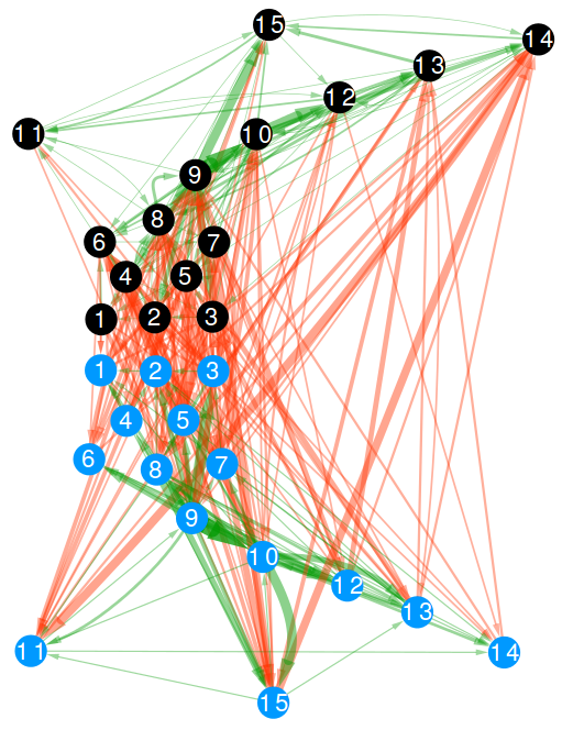
A passage network is simply a network whose nodes are the players of a team and the directed connections go from the player originating a pass to the player receiving the ball. We consider only completed passages: the ones that did not result in an error or lost possession. In the above picture, those are the green edges and they are always established between players belonging to the same team. In rugby, players are allowed to tackle the current ball carrier of the opponent team. When that happens, we create another directed edge, this time in what we call “disruption network”. The aim of a tackle is to prevent the opponent team from gaining meters. These are the red edges in the above picture and can only be established between players belonging to opposite teams. The picture you see is the collection of all passes and tackles which happened in the Italy vs New Zealand match in 2012. It is a multilayer network as it contains edges of two different types: passes and tackles.

Once we have pass and disruption networks we can calculate a collection of network measures. I’ll give a brief idea here, but if you are looking for more formal definitions you’ll have to search for them in the paper:

  • Connectivity: how many pass connections you have to remove to isolate players;
  • Assortativity: the tendency of players to pass the ball to players with a similar number of connections — in high assortativity central players pass to other central players and marginal players to other marginal players;
  • Components: how many “sinks” there are, in that the ball never goes back to the bulk of the team when it is passed to a player in a sink;
  • Clustering: how many triangles there are, meaning that the team can be decomposed in many different smaller sub-teams of three players.

These are the features we calculated for the pass networks. The disruption case is slightly different. We calculated the same features for the team when removing the tackled player, weighted on the relative number of tackles. If 50% of the tackles hit player number 11, then 50% of the disrupted connectivity is the connectivity value of the pass network when removing player 11. The reason is that the tackled player is temporarily removed from the game, so we need to know how the team performs without him, weighted on the number of times this occurrence happens.

So, it is time to give some answers. Shall we?

1. Is there a relationship between the topology of the network of passes and the success of the team?

rugby2

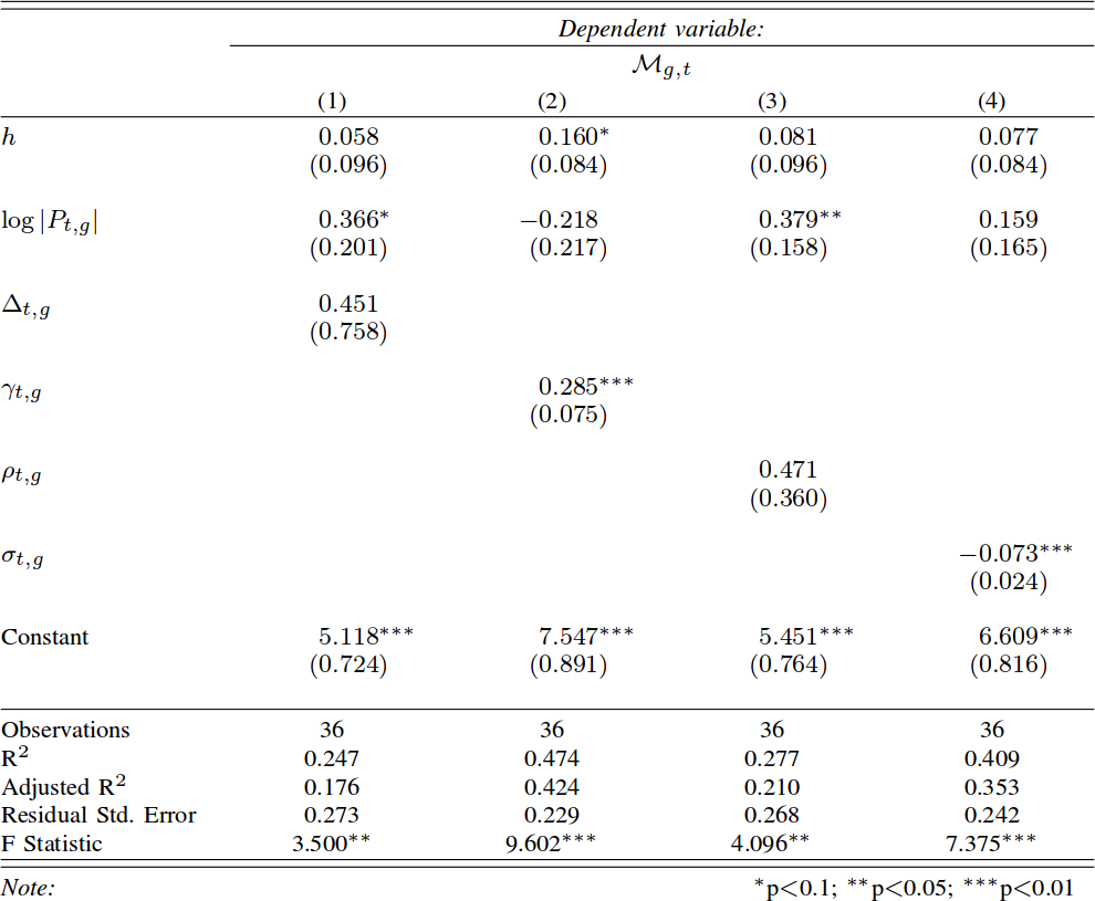
Yes, there is. We calculate “success” as the number of meters gained, ball in hand, by the team. The objective of rugby is to cross the goal line carrying the ball, so meters made is a pretty good indicator. We control for two things. First, the total number of passes: it simply means the team was able to hold onto the ball longer, so it is trivially expected to result in more meters. Second, the home advantage, which is a huge factor in rugby: Italy won only 12 out of 85 matches in the European “Six Nations” tournament, and 11 of them were in Italy. After these controls, we find that two features have good correlations with meters made: connectivity and components. The more edges are needed to isolate a player, the more meters a team is expected to make (p < .01, R2 = 47%). More sinks in a team is associated with lower gains in meters.

2. Is there a relationship between disruptions made by tackles and territorial gains?

rugby3

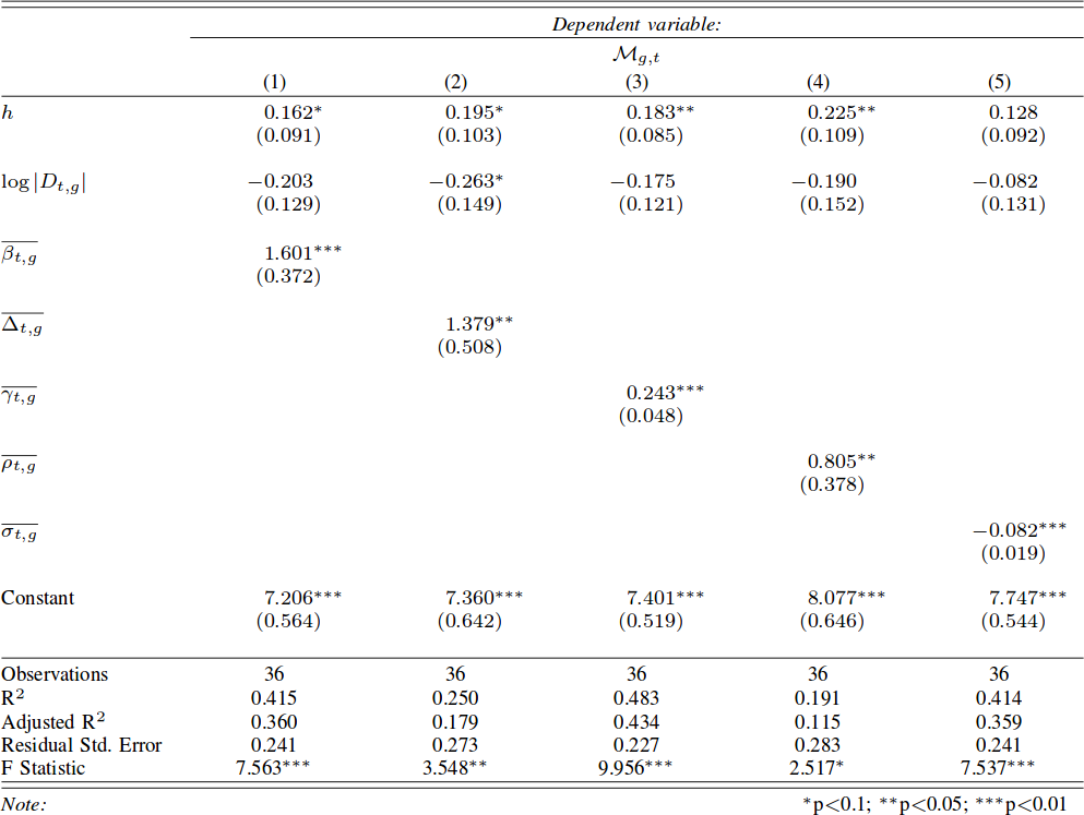
Again: yes. In this case it seems that all calculated features matter to predict meters made. The strongest factor is again leftover connectivity. It means that if the connectivity of the pass network increases after the tackled player is removed from it then the team is able to advance more. Simplifying: if you are able to tackle only low connectivity players, then your opponent is able to gain more territory (p < .01, R2 = 48%).

3. Is it better to build networks of passes and disruptions for each action separately or for the entire match?

The answer to the previous two questions were made by calculating the features on the global match networks. The global network uses all the data from a match, exactly like the pass and disruption edges depicted in the above figure. In principle, one could calculate these features as the match unfolds: sequence by sequence. In fact, networks features at the action level work very well in soccer, as Luca and Paolo already proved. Does that work also in rugby?

Surprisingly, the answer is no. We recalculated the features for each passage of play. A passage of play is the part of a match from when a team gets into possession of the ball until it loses it, scores, or the game flow stops for an infraction. When we calculate features at this level, we find very weak correlations: almost nothing is significant and, when it is, the predictive power is very low. We think that this is because in rugby our definition of sequence is too strict. While soccer is a tactical game — where each sequence counts for itself — rugby is a grand strategy game: sequences build cumulative advantage which pays off after a series of them — or only in the match as a whole.

4. Can we use these relationships to “predict” the outcome of the match?

mca_3099866b

This is the real queen question of the post, and we do not fully answer it, unfortunately. However, we have a very good reason to think that the answer could be positive. We created a predictor which trains on 17 matches and then, given the global multi-layer network, will pick the winner. You can see the problem of the approach here: we use the network of the match as it happened to “predict” the outcome. However, we did that only because we did not have enough matches for each individual team: we believe we can first predict how pass and disruption networks will shape in a new match using historic data and then use that to predict the outcome. That will be future works, maybe if some team is intrigued by networks and wants to contact us for a collaboration… (wink wink).

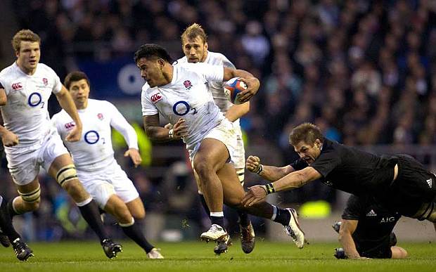
The reason I still like to report on our predictor is that it has a very promising property. Its accuracy was 83%. We compared with a prediction made with official rugby rankings, whose performance is worse: 76% accuracy. We also tested against bookmakers, who are better than us with their 86% accuracy. However, historic data on bets only cover more important matches — only 14 out of 18 — and matches between minor teams are usually less predictable. The fact that we are on par on a more difficult task is remarkable. More importantly, bookies tend to just “choose the best team”. For instance, they always predict a New Zealand win. The Haka, however, is not always enough and our networks caught that. New Zealand lost to England in a big upset on December 1st 2012. The bookmakers didn’t see that coming, but our network approach could have.

Continue Reading

24 April 2014 ~ 1 Comment

Data: the More, the Merrier. Right? Of Course Not

You need to forgive me for the infamous click-bait title I gave to the post. You literally need to, because you have to save your hate for the actual topic of the post, which is Big Data. Or whatever you want to call the scenario in which scientists are flooded with so much data that traditional approaches break, for one reason or another. I like to use the Big Data label just because it saves time. One of the advantages of Big Data is that it’s useful. Once you can manage it, simple analysis will yield great profits. Take Google Translate: it does not need very sophisticated language models because millions of native speakers will contribute better translations, and simple Bayesian updates make it works nicely.

Of course there are pros and cons. I am personally very serious about the pros. I like Big Data. Exactly because of that love, honesty pushes me to find the limits and scrutinize the cons of Big Data. And that’s today’s topic: “yet another person telling you why Big Data is not such a great thing (even if it is, sometimes)” (another very good candidate for a click-bait title). The occasion for such a shameful post is the recent journal version of my work on human mobility borders (click for the blog post where I presented it). In that work we analysed the impact of geographic resolution on mobility data to locate the real borders of human mobility. In this updated version, we also throw temporal resolution in the mix. The new paper is “Spatial and Temporal Evaluation of Network-Based Analysis of Human Mobility“. So what does the prediction of human mobility have to do with my blabbering about Big Data?

Big Data is founded on the idea that more data will increase the quality of results. After all, why would you gather so much data at the point of not knowing how to manage them if it was not for the potential returns? However, sometimes adding data will actually decrease the research quality. Take again the Google Translate example: a non native speaker could add noise, providing incorrect translations. In this case the example does not really hold, because it’s likely that the vast majority of contributions comes from people who are native speakers in one of the two languages involved. But in my research question about human mobility it still holds. Remember what was the technique in the paper: we have geographical areas and we consider them nodes in a network. We connect nodes if people travel from an area to another.

Let’s start from a trivial observation. Weekends are different from weekdays. There’s sun, there’s leisure time, there are all those activities you dream about when you are stuck behind your desk Monday to Friday. We expect to find large differences in the networks of weekdays and in the networks of weekends. Above you see three examples (click for larger resolution). The number of nodes and edges tells us how many areas are active and connected: there are much fewer of them during weekends. The number of connected components tells us how many “islands” there are, areas that have no flow of people between them. During weekends, there are twice as much. The average path length tells us how many connected areas you have to hop through on average to get from any area to any other area in the network: higher during weekdays. So far, no surprises.

If you recall, our objective was to define the real borders of the macro areas. In practice, this is done by grouping together highly connected nodes and say that they form a macro area. This grouping has the practical scope of helping us predict within which border an area will be classified: it’s likely that it won’t change much from a day to another. The theory is that during weekends, for all the reasons listed before (sun’n’stuff), there will be many more trips outside of a person’s normal routine. By definition, these trips are harder to predict, therefore we expect to see lower prediction scores when using weekend data.

The first part of our theory is proven right: there are indeed much less routine trips during weekends. Above we show the % of routine trips over all trips per day. The consequences for border prediction hold true too. If you use the whole week data for predicting the borders of the next week you get poorer prediction scores. Poorer than using weekday data for predicting weekday borders. Weekend borders are in fact much more volatile, as you see below (the closer the dots to the upper right corner, the better the prediction, click for higher resolution):

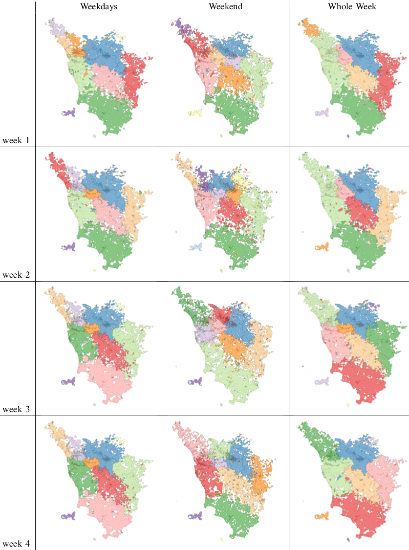
In fact we see that the borders are much crazier during weekends and this has a heavy influence on the whole week borders (see maps below, click for enjoying its andywarholesque larger resolution). Weekends have a larger effect on our data (2/7), much more than our example in Google Translate.

maps

The conclusion is therefore a word of caution about Big Data. More is not necessarily better: you still need theoretical grounds when you add data, to be sure that you are not introducing noise. Piling on more data, in my human mobility study, actually hides results: the high predictability of weekday movements. It also hides the potential interest of more focused studies about the mobility during different types of weekends or festivities. For example, our data involves the month of May, and May 1st is a special holiday in Italy. To re-ignite my Google Translate example: correct translations in some linguistic scenarios are incorrect otherwise. Think about slang. A naive Big Data algorithm could be caught in between a slang war, with each faction claiming a different correct translation. A smarter, theory-driven, algorithm will realize that there are slangs, so it will reduce its data intake to solve the two tasks separately. Much better, isn’t it?

Continue Reading

28 February 2013 ~ 0 Comments

Networks and Eras

The real world has many important characteristics. One I heard being quite salient is the fact that time passes. Any picture of the world has to evolve to reflect change, otherwise it is doomed to be representative only of a narrow moment in time. This is quite a problem in computer science, because when we want to analyze something we need to spend a lot of time in gathering data and, usually, the analysis can be done only once we have everything we need. It’s a bit like in physics, when the problems are solved in the vacuum and in the absence of friction. Of course, many people work to develop dynamics models, trying to handle the changes in the data.

Take link prediction, for example. Link prediction is the branch of network science whose aim is to predict which connections are more likely to appear in the near future, given the current status of a network. There are many approaches to this problem: one simply states that the probability that two nodes will connect is proportional to their current degree (because it’s being observed that high degree nodes attracts more edges, it’s called “preferential attachment“), another looks at the history of the new edges which came into existence and tries to redact some evolution rules (see the paper, not much different from my work on signed networks).

What’s the problem in this? The problem lies in the fact that any link came into existence in a specific moment, in which the network shape was different from any other moment. Let’s consider the preferential attachment, with an example. The preferential attachment tells you that the position in the market of Google not only is not in danger: it will become stronger and stronger, because its high visibility attracts everybody who needs the services it is providing. However, Google was not born with the web, but several years after. So in the moment in which Google was born, the preferential attachment would have told you that Google had no chance to beat Yahoo. And now it’s easy to laugh at this idea.

So, what happened? The idea that I investigated with my colleagues at the KDDLab in Italy is extremely simple: just like Earth’s geological times, also complex networks (and complex systems in general) evolve discontinuously, with eras in which some evolution rules apply and some others, valid in other eras, don’t. The original paper is quite old (from 2010), but we recently published an update journal version of it (see the Intelligent Data Analysis Journal), that’s why I’m writing about it.

In our paper, we describe how to build a framework to understand what are the eras in the evolution of a network. Basically, everything boils down to have many snapshots of the network in different moments of time and a similarity measure that tells you how similar are two consecutive snapshots. Then, by checking the values of this similarity function, one can understand if the last trends she is seeing are providing reliable information to make predictions or not. In our world, then, we understand that when Google enters in the web anything can happen, because we are in a new era and we do not use outdated information that do not apply anymore to the new scenario. In our world, also, we are aware that nobody is doomed to success, regardless how good its current position is. A nice and humbling perspective, if I may say.

I suggest reading the paper to understand how nicely our era detection system fits with the data. The geekier readers will find a nice history of programming languages (we applied the era discovery system to the network of co-authorship in computer science), normal people will probably find more amusement in our history of movies (from networks of collaboration extracted from the Internet Movie Database).

So, next time you’ll see somebody trying to make predictions using complex network analysis, check if she is considering data history using an equivalent of our framework. If she does, thumbs up. If she doesn’t, trust her just like you would trust a meteorologist trying to forecast tomorrow’s weather by crunching data from yesterday down to the Mesozoic.

Continue Reading