Michele Coscia

New year, old topic. I could make a lot of resolutions for this new year, but for sure to stop talking about community discovery is not among them. At least this time I tried to turn it up a notch in the epicness of the title. My aim is to give some substance to one of the many typical filler phrases in science writing. The culprit sentence in this case is “different application scenarios demand different approaches”. Bear with me for a metaphoric example.

When presenting a new toaster, it is difficult to prove that it toasts everything better under any point of view, under any circumstances. It usually does most toasts okay, and for one kind of toasts it really shines. Or its toasts really suck, but it can toast underwater. That’s fine. We are all grown up here, we don’t believe in the fairy tales of the silver bullets any more. At this point, our toaster salesman is forced to say it. “Different application scenarios demand different approaches”. In some cases this is a shameful fig leaf, but in many others it is simply true. Problem is: nobody really checks.

I decided to check. At least one of them. Teaming up with Diego Pennacchioli and Dino Pedreschi, I put the spotlight on one of the strongest dichotomies in community discovery.  As you may remember, community discovery algorithms can force every node to belong to just one community, or allow them to be in many of them. The former approach is called “graph partitioning”, whilst the latter aims to find an “overlapping coverage”. Are these two strategies yielding interesting, yet completely different, results? This question has been dissected in the paper: “Overlap Versus Partition: Marketing Classification and Customer Profiling in Complex Networks of Products“, that will be presented in one workshop of the 2014 edition of the International Conference of Data Engineering.  Let me refresh your mind about overlaps and partitions.

Above you have the nec plus ultra scenario for a partitioning algorithm. If a partitioning algorithm sees the graph on the left, it would just die of happiness. In the graph, in fact, it appears very clearly that each node belongs to a very specific community. And it can’t belong to any other. If we assume that our algorithm works on edge strength (e.g. the inverse of the edge betweenness), then what the algorithm really sees is the graph on the right. It then proceeds to group together the nodes for which the edge strength is maximal, et voilà.

Here we have an example that’s a bit more complex. The picture has too many overlapping parts, so let me describe the connection pattern. In the graph on the left there are several groups of 6 nodes, each node connected to all other members of the group. In practice, each diagonal is completely connected to the two neighbouring diagonals. Clearly, here there is no way we can put each node in a disjoint group. Why put together nodes 0,1,2 with 3,4,5 and not with 9,10,11? But at that point, why 9,10,11 should be in a community with them and not with 6,7,8? The correct approach is just to allow every completely connected group to be a community, thus letting nodes to be part of more than a community. Some overlapping algorithms see the graph as it has been depicted on the right, with an edge colour per densely connected group.

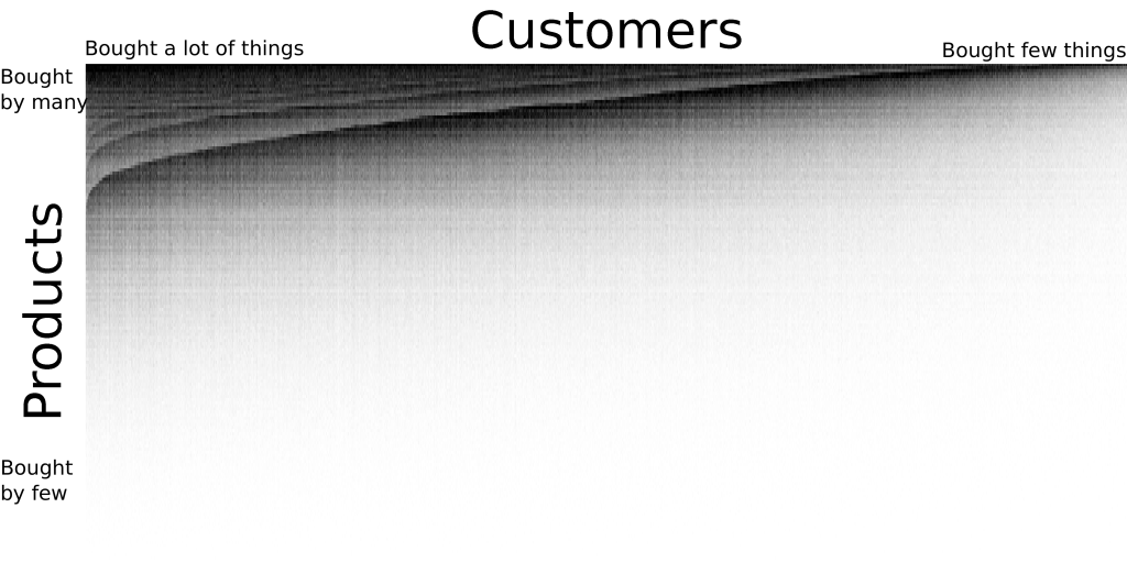
Time to test which one of these approaches is The Right One! For our data quest we focused on supermarket transactions. We created a network of products that you can buy in supermarkets. To be connected, two products have to be bought together by the same customers in a significant number of times. What does that mean? By pure intuition, bread and water aren’t going to be connected: both of them are bought very frequently, but they have little to do with each other, thus they are expected to be in the same shopping cart by chance. Eggs and flour are too very popular, but probably more than chance, since there are a lot of things you can do with them together. Therefore they are connected. Other specific pairs of products, say bacon flavoured lipstick and liquorice shoelaces, may ended up in the same, quite weird, shopping cart. But we don’t connect them, as their volume of sales is too low (or at least I hope so).

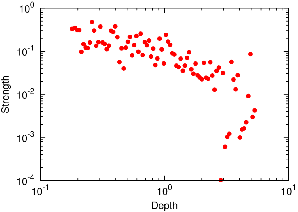
Here are some of the facts we found. First. The overlapping approach* tends to return relatively more communities with a larger amount of nodes than the partition approach**. In absolute terms that’s obvious, since the same node is counted more than once, but here the key term is “relatively”. See the plot above on the right, where we graph the probability (y axis) of finding a community with a given number of nodes (x axis). Second. The overlapping approach returns more “messy” communities. Our messiness measure checks how many different product categories are grouped together on average in the same community. Again, larger communities are expected to be messier, but the messiness measure that we used controls for community size. See the plot on the right, again the probability (y axis) of finding a community with a given entropy (x axis, “entropy” is the fancy scientific term for “messiness”). Third. The partition approach returned denser communities, whose link strength (the number of people buying the products together) is higher.

What is the meaning of all this? In our opinion, the two algorithms are aiming to do something completely different. The partition approach is aiming to create a new marketing classification. It more or less coincides with the established one (thus lower messiness), most customers buy those products together (high link strength) and there are very few giant categories (most communities are small). The overlapping approach, instead, wants to do customer profiling. A customer rarely buys all products of a marketing category (thus increasing its messiness), it has specific needs (that not many people have, thus lowering edge weight) and she usually needs a bunch of stuff (thus larger communities, on average).

Who’s right? That’s the catch: both. The fact that two results are incompatible, in this case, does not mean that one is right and one is wrong. They are just different applications. Which was exactly what I wanted to prove, in this narrow and very specific, probably unsurprising, scenario. Now you should feel better: I gave you a small proof that the hours you spend to choose the perfect toaster for you are really worth your time!

* As overlapping approach, we used the Hierarchical Link Clustering.

** As partitioning approach, we used Infomap.

Continue Reading

“It’s a bit sad that some among the most brilliant minds of our generation are working tirelessly on strategies to increase clicks on online ads” popped up on my Facebook stream some days ago (I don’t remember who wrote it, so you are welcome to contact me to restore credit where credit is due 🙂 ). But the point still remains. I actually don’t find it that bad. Yes, it’s bad, but it could be worse. It reminds me of other “wrong” reasons to do incredible improvements in science and stuff. For example, war is responsible for many technology advancements. Even if the aim of online marketing is just to increase revenues, what it actually requires is to understand human psychology, behavior and social interactions. In practice, that’s philosophy of the human mind at its best: how does the brain work? How does a collection of brains work? What drives our behavior and needs?

When you put together many minds in the real world, you have to deal with complex networks. We are not connected with one another at random, and the eyes of our friends are the channel through which we observe the world. This fact is studied in complex network analysis, in the sub-branch of cascade behaviors. Cascade behaviors happen when a person in a social network decides to modify her behavior according to the behavior of the people she is connected to. As a consequence, there are some people in the network who are in a very particular position: given the people they know and their prominence among them, they can modify their behavior and they will modify their friends’ behavior and so on an so forth, changing forever how every node in the network behaves. And that’s the cascade. If you find a way to identify these prominent actors in the network, you can control the behavior of the entire system. Now you can see why there is a mountain of work about it. In the computer science approach, we have threshold models simulating the cascade for many starting nodes and thus identify the practical leaders (for example Jon Kleinberg’s work); in physics we have models, aiming at understanding the degree of controllability of complex systems (I’ll go with Laszlo Barabasi in this).

Visualization of network cascade, from my good friend Mauro Martino. The red dots at the bottom are the “drivers”, who influence the collection of green nodes they are attached to.

Genuinely curious about the topic, I started my own track of research on it. One thing that Diego Pennacchioli, Giulio Rossetti, Luca Pappalardo, Dino Pedreschi, Fosca Giannotti and me found curious is that everybody working on social prominence was looking at it from a monodimensional perspective. That means: the only thing they are interested in is how to maximize the number of nodes influenced by the leaders. The bigger this number, the better. All fun and games, but why? I can think about several scenarios where the final total number is not the most important thing. For example:

• What if I want people to buy a product? The total number of people knowing about the product is nice, but I want them to be strongly committed, strongly enough to buy it.
• What if I am actually looking to reach a particular person? Then I care how deeply my message can go through the network.
• What if I just care about my friends? Then screw their friends (and everybody else), as long as I can influence a wide range of my direct connections!

To calculate our measure we need to infer the diffusion trees. So from the left, where the number on each arrow gives you the action time of the node at the base of the arrow, we go to the right by selecting the lowest possible combination of arrows.

Strength, depth and width of social prominence. That’s why our paper is called “The Three Dimensions of Social Prominence” (check it out). Strength is how committed the people you influenced are to keep doing what you influenced them to do. Depth is how many degrees of separation (or, how far) the cascade of influence that you triggered can go. Width is simply the ratio of your friends that you are able to influence. By analyzing how much a user in Last.fm (a social website based on music) is able to influence her friends in listening to new artists, we found a collection of very interesting facts.

For example, it is well known that in social networks there are some nodes that are structurally very important. They are the central users, the ones that keep the network connected. Intuitively, they are the only way, or the easiest way, through which a signal (in our case social influence) can go from one part of the network to the other. Guess what: they can’t do it. We found a significant anti-correlation between centrality and width and depth. That is bad news, because those nodes are the ones in the only position with a theoretical ability of controlling the network and a practical inability in doing so. I like to call it “The Paradox of Social Controllability” (hence, the post title).

The anti-correlation between depth and strength.

Another piece of food for thought is the trade off between strength and depth. While width is unrelated to both, we found that if you want to go deeply into the network, then you can’t expect that the people you touch will be extremely committed to your message.

The third big thing is the distribution of connections per leader. We found that the leaders showing highest values of strength, depth and width were those who used Last.fm with average frequency. The highly connected and very active users (hubs, in network lingo) scored poorly, as we saw. So did the occasional users, the ones with just two or three connections (that is the majority of the system). The people who have control over the network are the mildly engaged. They are you, in practice: chances are that you are not a record label, nor a music fanatic, but just a person with her tastes and preferences. So you have control. Problem is, the control is scattered equally on the vast set of people like you.

To conclude, we saw what wonderful things network cascades are: they could empower us to do a lot of good. We also saw how there are theoretical results about the possibility of identifying people who can trigger them. But my unfortunate conclusion is about the paradox between theory and practice. Those who theoretically should, apparently can’t.

Continue Reading

The Holy Grail of every marketing system is to understand how the mind of the customers works. For example answering the question: “From how far can I attract customers?” To do so means to increase profits. You can deploy your communication and products more efficiently and maximize your returns. Clearly, there is no silver bullet for this task. There is no way that one single aspect is so predominant in a person’s mind at the point of empowering a seller to have perfect control over who will buy her product, where and when. If that would be true, there would be no space left for marketing specialists, demand segmentation and so on. Many little tricks can be deployed in the market.

I am by no means an expert on the field, so my way to frame this problem may sound trivial. In any case, I can list three obvious parameters that affect a customer’s decision in buying or not buying a product. The first is price. Few people want to throw their money senselessly, most of them want to literally maximize the bang for their buck (okay, maybe not that literally). The second is the quantities needed: if I need to buy product X everyday in large bulks and product Y once in a blue moon, then it’s only fair to assume that I’ll consider different parameters to evaluate X and Y.

The third is the level of sophistication of a given product. There are things that fewer and fewer people need: birdseed, piña colada flavored lip balm. Narrower customer base means less widespread offer, thus the need of travel more to specialized shops. Intuitively, sophistication is more powerful than price and quantity: a Lamborghini is still a car – also quite useless when doing groceries – like a Panda, but it satisfies very different and much more sophisticated needs. Sophistication is powerful because you can play with it, increasing the perceived sophistication of a product, thus your market: like Jonah Berger‘s  “thee types of ice” bar, that looked more fancy just by inventing a way to make ice sound more sophisticated than it is.

So let’s play and try to use these concepts operatively. Say we want to predict the distance a customer is willing to travel to buy a product. Then, we try to predict such a distance using different variables. The one leading to better predictions of these distances wins as the best variable describing what motivates a customer to travel. We decided to test the three variables I presented before: price, quantity and sophistication. In this theory, higher prices mean longer distances to travel, as if I have to buy an expensive TV I’ll probably go around and check where is the best quality-price ratio. Higher quantities mean shorter distances, as if I have to buy bread everyday I don’t care where the best bakery of the city is if that means traveling ten kilometers everyday. Finally, higher sophistication means longer distances: if I have sophisticated needs I need to travel a lot to satisfy them.

Price and quantity are easy to deal with: they are just numbers. So we can put them on the X axis of a plot and put the distance traveled on the Y axis. And that’s what we did, for price:

and for quantity:

Here, each dot is a customer buying a product. If the dots had the same distance and the same price/quantity then we merged them together (brighter color = more dots here). We see that our theory, while not perfect, is correct: higher prices means longer distances traveled, higher quantities means shorter distances. Time to test for the level of sophistication! But now we hit a brick wall. How on earth am I suppose to measure the level of sophistication of a person and of a product? Should I split the brain of that person in half? How can I do this for thousands or millions of customers? We need to invent a brain splitting machine.

That’s more or less what we did. In a joint work with Diego Pennacchioli, Salvo Rinzivillo, Fosca Giannotti and Dino Pedreschi, that will appear in the BigData 2013 conference (you can download the paper, if you are interested), we proposed such a brain slice device. Of course I am somewhat scared by all the blood that would result in literally cutting open thousands of skulls, so we implemented a data mining machine that just quantifies with a number the level of sophistication of a customer’s needs and the level of sophistication that a product can satisfy, solving the issue at hand with no bloodshed.

The fundamental question is: is the level of sophistication a number? Intuition would tell us “no”: it’s a complex multidimensional space and my needs are unique like a snowflake. Kind of. But with a satisfying level of approximation, surprisingly, we can describe sophistication with a number. How is that possible? A couple of facts we discovered: customers buying the least sold products also buy everything else (the “simpler” stuff), and products bought just by few customers are bought only by those who also buy everything else. In other words, if you draw a matrix connecting the customers with the products they buy, this matrix is nested, meaning that all purchases are in the top left corner:

A-ha! Then it’s fair to make this assumption: customers are adding an extra product bought only if they already buy (almost) everything else “before” it. This implies two things: first, is that they add the extra product if all their previous products already satisfied their more basic needs (then, they are more sophisticated); second, is that they are moving on a monodimensional space, adding stuff incrementally. Then, they can be quantified by a number! I won’t go in the boring details about how to calculate this number. Suffice to say that they are very similar to how you calculate a country’s complexity, about which I wrote months ago; and that this number is not the total amount of money they spend, nor the quantity of products they buy.

So, how does this number relate to the distance traveled by customers?

The words you are looking for is “astonishingly well”.

So our quantification of the sophistication level has a number of practical applications. In the paper we explore the task of predicting in which shop a customers will go to buy a given product. We are not claiming that this is the only important factor. But it gives a nice boost. Over a base accuracy of around 53%, using the price or the quantity gives you a +6-7% accuracy. Adding the sophistication level gives an additional +6-8% accuracy (plots would suggest more, but they are about continuous numbers, while in reality shop position is fixed and therefore a mistake of a few hundreds meters is less important). Not bad!

Continue Reading