Michele Coscia

Ideological polarization is the tendency of people to hold more extreme political opinions over time while being isolated from opposing points of view. It is not a situation we would like to get out of hand in our society: if people adopt mutually incompatible worldviews and cannot have a dialogue with those who disagree with them, bad things might happen — violence, for instance. Common wisdom among scientists and laymen alike is that, at least in the US, polarization is on the rise and social media is to blame. There’s a problem with this stance, though: we don’t really have a good measure to quantify ideological polarization.

This motivated Marilena Hohmann and Karel Devriendt to write a paper with me to provide such a measure. The result is “Quantifying ideological polarization on a network using generalized Euclidean distance,” which appeared on Science Advances earlier this month.

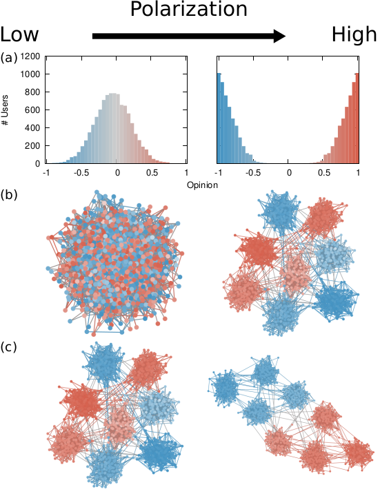
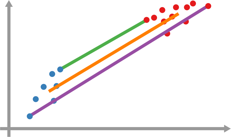
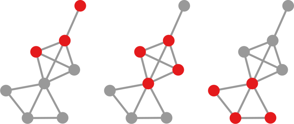
Our starting point was to stare really hard at the definition of ideological polarization I provided at the beginning of this post. The definition has two parts: stronger separation between opinions held by people and lower level of dialogue between them. If we look at the picture above we can see how these two parts might look. In the first row (a) we show how to quantify a divergence of opinion. Suppose each of us has an opinion from -1 (maximally liberal) to +1 (maximally conservative). The more people cluster in the middle the less polarization there is. But if everyone is at -1 or +1, then we’re in trouble.

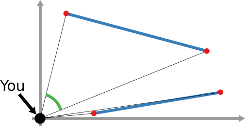
The dialogue between parts can be represented as a network (second row, b). A network with no echo chambers has a high level of dialogue. As soon as communities of uniform opinions arise, it is more difficult for a person of a given opinion to hear the other side. This dialogue is doubly difficult if the communities themselves organize in the network as larger echo chambers (third row, c): if all communities talk to each other we have less polarization than if communities only engage with other communities that hold more similar opinions.

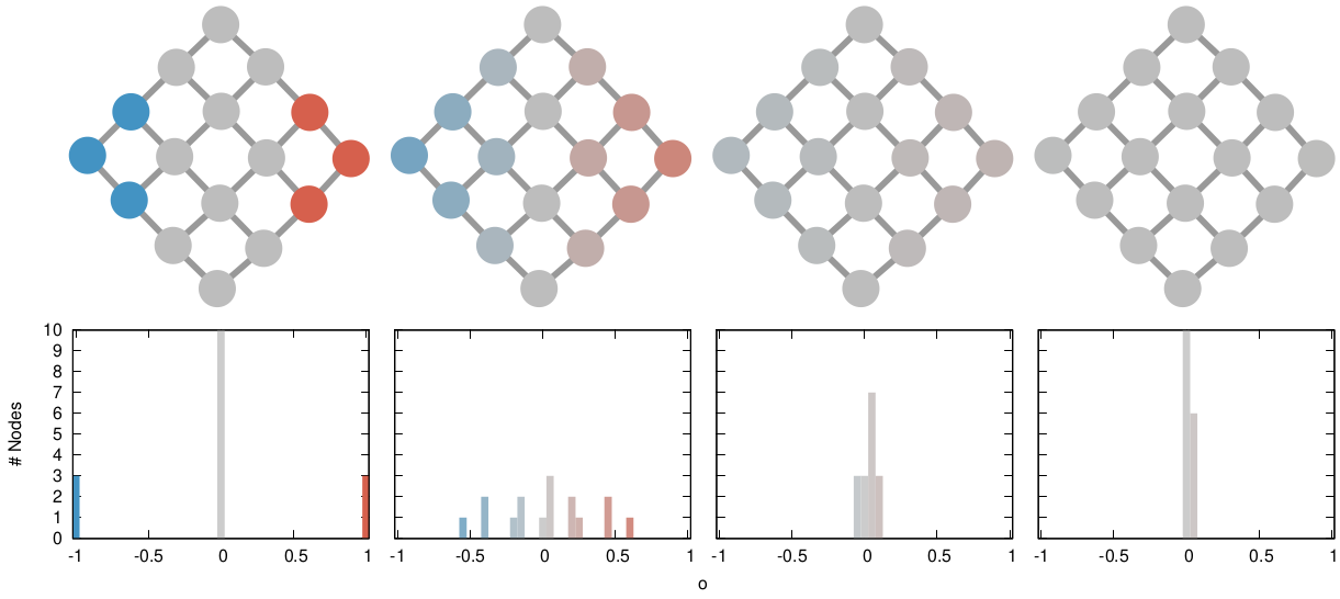
The way we decided to approach the problem was to rely on the dark art spells of Karel, the Linear Algebra Wizard to simulate the process of opinion spreading. In practice, you can think the opinion value of each person to be a certain temperature, as the image above shows. Heat can flow through the connections of the network: if two nodes are at different temperatures they can exchange some heat per unit of time, until they reach an equilibrium. Eventually all nodes converge to the average temperature of the network and no heat can flow any longer.

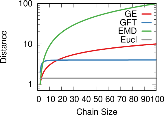
The amount of time it takes to reach equilibrium is the level of polarization of the network. If we start from more similar opinions and no communities, it takes little to converge because there is no big temperature difference and heat can flow freely. If we have homogeneous communities at very different temperature levels it takes a lot to converge, because only a little heat can flow through the sparse connections between these groups. What I describe is a measure called “generalized Euclidean distance”, something I already wrote about.

There are many measures scientists have used to quantify polarization. Approaches range from calculating homophily — the tendency of people to connect to the individuals who are most similar to them –, to using random walks, to simulating the spread of opinions as if they were infectious diseases. We find that all methods used so far are blind and/or insensitive to at least one of the parts of the definition of ideological polarization. We did… a lot of tests. The details are in the paper and I will skip them here so as not to transform this blog post into a snoozefest.

Once we were happy with a measure of ideological polarization, we could put it to work. The image above shows the levels of polarization on Twitter during the 2020 US presidential election. We can see that during the debates we had pretty high levels of polarization, with extreme opinions and clear communities. Election night was a bit calmer, due to the fact that a lot of users engaged with the factual information put out by the Associated Press about the results as they were coming out.

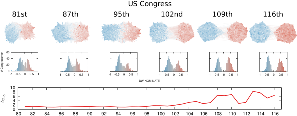
We are not limited to social media: we can apply our method to any scenario in which we can record the opinions of a set of people and their interactions. The image above shows the result for the US House of Representatives. Over time, congresspeople have drifted farther away in ideology and started voting across party lines less and less. The network connects two congresspeople if they co-voted on the same bill a significant number of times. The most polarized House in US history (until the 116th Congress) was the 113th, characterized by a debt-ceiling crisis following the full application of the Affordable Care Act (Obamacare), the 2014 Russo-Ukrainian conflict, strong debates about immigration reforms, and a controversial escalation of US military action in Syria and Iraq against ISIS.

Of course, our approach has its limitations. In general, it is difficult to compare two polarization scores from two systems if the networks are not built in the same way and the opinions are estimated using different measures. For instance, in our work, we cannot say that Twitter is more polarized than the US Congress (even though it has higher scores), because the edges represent different types of relations (interacting on Twitter vs co-voting on a bill) and the measures of opinions are different.

We feel that having this measure is a step in the right direction, because at least it is more accurate than anything we had so far. All the data and code necessary to verify our claims is available. Most importantly, the method to estimate ideological polarization is included. This means you can use it on your own networks to quantify just how fu**ed we are the healthiness of our current political debates.

Continue Reading

We all know that correlation doesn’t imply causation:

And yet, we calculate correlations all the time. Because knowing when two things correlate is still pretty darn useful. Even if there is no causation link at all. For instance, it’d be great to know whether reading makes you love reading more. Part of the answer could start by correlating the number of books you read with the number of books you want to read.

As a network scientist, you might think that you could calculate correlations of variables attached to the nodes of your network. Unfortunately, you cannot do this, because normal correlation measures assume that nodes do not influence each other — the measures are basically assuming the network doesn’t exist. Well, you couldn’t, until I decided to make a correlation coefficient that works on networks. I describe it in the paper “Pearson Correlations on Complex Networks,” which appeared in the Journal of Complex Networks earlier this week.

The formula you normally use to calculate the correlation between two variables is the Pearson correlation coefficient. What I realized is that this formula is the special case of a more general formula that can be applied to networks.

In Pearson, you compare two vectors, which are just two sequences of numbers. One could be the all the numbers of books that the people in our sample have read, and the other one is all of their ages. In the example, you might expect that older people had more time to read more books. To do so, you check each entry in the two vectors in order: every time you consider a new person, if their age is higher than the average person’s, then also the number of books they read should be higher.

If you are in a network, each entry of these vectors is the value of a node. In our book-reading case, you might have a social network: for each person you know who their friends are. Now you shouldn’t look at each person in isolation, because the numbers of books and the ages of people also correlate in different parts of the network — this is known as homophily. Some older people might be pressured into reading more books by their book-addicted older friends. Thus, leaving out the network might cause us to miss something: that a person’s age tells us not just about the number of books they have read, but it also allows us to predict the number of books their friends have read.

To put it simply, the classical Pearson correlation coefficient assumes that there is a very special network behind the data: a network in which each node is isolated and only connects to itself — see the image above. When we slightly modify the math behind its formula, it can take into account how close two nodes are in the network — for instance, by calculating their shortest path length.

You can interpret the results from this network correlation coefficient the same way you do with the Pearson one. The maximum value of +1 means that there is a perfect positive relation: for every extra year of age you read a certain amount of new books. The minimum of -1 means that there is a perfect negative relationship: a weird world where the oldest people have not read much. The midpoint of 0 means that the two variables have no relation at all.

Is the network correlation coefficient useful? Two answers. First: how dare you, asking me if the stuff I do has any practical application. The nerve of some people. Second: Yes! To begin with, in the paper I build a bunch of artificial cases in which I show how the Pearson coefficient would miss correlations that are actually present in a network. But you’re not here for synthetic data: you’re a data science connoisseur, you want the real deal, actual real world data. Above you can see a line chart, showing the vanilla Pearson (in blue) and the network-flavored (in red) correlations for a social network of book readers as they evolve over time.

The data comes from Anobii, a social network for bibliophiles. The plot is a correlation between number of books read and number of books in the wishlist of a user. These two variables are positively correlated: the more you have read, the more you want to read. However, the Pearson correlation coefficient greatly underestimates the true correlation, at 0.25, while the network correlation is beyond 0.6. This is because bookworms like each other and connect with each other, thus the number of books you have read also correlates with the wishlist size of your friends.

This other beauty of a plot, instead, shows the correlation between the age of a user and the number of tags they used to tag books. What is interesting here is that, for Pearson, there practically isn’t a correlation: the coefficient is almost zero and not statistically significant. Instead, when we consider the network, there is a strong and significant negative correlation at around -0.11. Older users are less inclined to tag the books they read — it’s just a fad kids do these days –, and they are even less inclined if their older friends do not tag either. If you were to hypothesize a link between age and tag activity and all you had was lousy Pearson, you’d miss this relationship. Luckily, you know good ol’ Michele.

If this makes you want to mess around with network correlations, you can do it because all the code I wrote for the paper is open and free to use. Don’t forget to like and subscrib… I mean, cite my paper if you are fed up with the Pearson correlation coefficient and you find it useful to estimate network correlations properly.

Continue Reading

Back in March I wrote a blog post — and a paper — showing a technique to estimate the distance covered by a propagation event on a network between two moments in time. A propagation event could be the failure of a power grid, a word-of-mouth campaign on social media, or — more topically these days — a disease infecting people in a social network. The limitation of that paper was in taking only a single perspective. However, this problem could be solved in at least a dozen different ways. To give justice to such complexity, I recently co-authored the paper “The Node Vector Distance Problem in Complex Networks” with Andres Gomez, James McNerney, and Frank Neffke. The paper was published this month in the ACM Computing Surveys journal and it’s the main focus of this blog post.

Estimating the spreading speed of something in our normal geographical space is important, but relatively trivial. However, networks are complex spaces. You cannot estimate the speed of COVID by looking at the geographical areas it has covered, because what really connects places is not our physical space, but a complex network of relations among regions. In other words, the places closest to China are not necessarily countries like Mongolia or Nepal — both of which share a border with China — but Iran and Italy, because of the many direct flights connecting them.

My paper in March found a way to transform our notion of Euclidean distance — a straight line in physical space — to networks. It basically defined what a “straight line” means when all you have is nodes and edges. In the figure above, I connect countries if they have a significant number of direct flights between their airports. Darker nodes represent countries that were hit earlier, and nodes get progressively lighter the later they were first hit. My generalized Euclidean measure allows you to calculate a number describing how fast this process went. This means you could compare it with other pandemics, or you could use it to estimate the moment when a still-developing pandemic will cover a given fraction of the world.

Was mine the only way to translate the concept of “straight line”? No. For starters, it uses an indirect metaphor to define “straightness”. In my generalized Euclidean, every node is a “dimension” of a multidimensional space and, when COVID infects it, it means that the virus had traveled a certain amount of distance in that dimension. If you’re staring dumbfounded at the previous sentence, yeah, that’s pretty much what I expected. A more intuitive way of defining the distance covered in a network would be simply to count how many edges the disease crossed via the calculation of shortest paths.

However, it’s still not that easy: how far is each newly infected node from the set of previous infected nodes? And how do we combine all those path lengths into one new measure? In the paper, we explain various ways to do so. One option is to apply linking strategies from hierarchical clustering, as I show in the figure above. The distance between the group of red points from the blue points can be the distance of their closest pair — green line, called single linkage –; the distance of their centers of mass — orange line, average linkage –; or the distance between their farthest pair — purple line, complete linkage. Another option is to simulate an agent optimizing the movement of “packets” from the nodes in the origin to the nodes in the destination — the popular Earth Mover’s Distance measure.

And that still doesn’t cover the space of possibilities! Even in our simple geographical world, we can have different perspectives on what “distance” means. For instance, a popular distance measure is cosine distance. In it, it doesn’t matter how far two points are in the space: if they are on the same line from your point of view, you consider them close together. Now, “distance” becomes the angle by which you have to turn to go from looking straight at one point, to looking at the other. In the figure below, the Euclidean (straight line) distance between two red points is in blue. The cosine distance is the thick green line, showing in the point pair below that it could be quite small even for points that Euclid would say are very far away in the plane. Many measures adopt this distance philosophy for networks, for instance the Mean Markov Chain and the Graph Fourier Transform approaches.

That is more or less where we stop in the paper. I think that there are plenty more network distance measures to be discovered, but the work still needs to be done.

As a companion for the paper, I have developed an open source Python library implementing the majority of network distance measures that we discuss. You can use it to calculate network distances in your data, or to better understand how these measures work. Hopefully, you’ll make my job harder by discovering new measures and forcing me to publish an updated paper on the topic.

Continue Reading

I don’t need to introduce to you what the corona virus is: COVID-19 has had a tremendous impact on everyone’s life in the past weeks and months. All of a sudden, our social media feeds have been invaded with new terminology: social distancing, R0, infection rate, exponential growth. Overnight, we turned ourselves into avid consumers of epidemics literature. We learned what the key to prevent the infection from becoming a larger problem is: slow the bugger down. That is why knowing how fast corona is actually moving is such a crucial piece of information. You have seen the pictures many times, they look something like this:

What you’re seeing is the evolution in number of infected people — and how much non-infected people like me blabber about them online. Epidemiologists try to estimate the speed of infection by fitting the real data you see on an SI model. In it, people turn from Susceptible to Infected at a certain rate. These models are usually precise at estimating the number of infected over time, but they lack a key component: they assume that each individual is interchangeable and that anyone has a chance to be infected by anyone in their close proximity. In other words, they ignore the fact that we are embedded in a social network: some people are more central than others, and some have more friends than others.

To properly estimate how fast a disease moves, you need to take the network into account. And this is the focus of a paper of mine: “Generalized Euclidean Measure to Estimate Network Distances“. The paper has been accepted for publication at the 2020 ICWSM conference. The idea of the paper is to create a new measure that estimates the distance between the state of the disease at two moments in time, taking the underlying network topology into account.

The question here is deceptively simple. Suppose you have a set of infected individuals. In the picture above, they are the nodes in red in the leftmost social network. After a while, some people recover, while others catch the disease. You might end up with the set of infected from the network in the middle, or the one in the right. In which case did the disease spread more quickly?

We have a clear intuitive answer: the rightmost network experienced a faster spread, because the infected nodes are farther from the original ones. We need to find a measure that matches this intuition. How do we normally estimate distances in the real world? We use a ruler: we draw a straight line between two points and we measure how long that line is. This is the Euclidean distance. Mathematically, that means representing the two points as vectors of coordinates (p and q), calculating their difference, and then using Pythagoras’ theorem to calculate the length of the straight line between them:

We cannot apply this directly to our network problem. This is because, for silly Euclid, every dimension has the same importance in estimating the distance between points. However, in our case, the points are the states of the disease. They do not live on the plane of Euclidean geometry, but on a network. Some moves in this network space are short and easy: moving between two connected nodes. But other moves are long and hard: between two nodes that are far apart. In other words, nodes that are connected to each other contribute less than unconnected nodes to the distance. The simplest example I can make is:

In the figure, each vector — for instance (1,0,0) — is the representation of the state of the disease of the graph beneath it: the entries equal to one identify the currently infected node. Clearly, the infection closer to the left graph is the middle one, not the right one. However, the Euclidean distance between the three vectors is the same: the square root of two. So how do we fix this problem? There is a distance measure that allows you to weigh dimensions differently. It is my favorite distance metric (yes, I am the kind of person who has a favorite distance metric): the Mahalanobis distance. Mahalanobis simply says that correlated variables should count less in estimating the distance: taller people tend to be heavier — because there’s more person to weigh — so we shouldn’t be surprised if someone taller than me is also heavier. But, if they weigh less, we would find it remarkable.

Now we’re just left with the problem of figuring out how to estimate, mathematically, what “correlated” means in a network. The paper has the full details. For here, suffice to say we augment Pythagoras’ theorem with the pseudoinverted graph Laplacian — a sentence I’m writing only to pretend I’m smart (it’s actually not sophisticated at all, and a super easy thing to calculate). The reason we use the graph Laplacian is because it is a standard instrument to estimate how fast things spread in a network.

In the paper I run a bunch of tests to show that this measure matches our intuition. For instance, as shown above, if we have infected people at the endpoints of a chain graph, the longer the chain (x axis) the higher the estimated distance should be (y axis). GE (= Generalized Euclidean, in red) is my measure, and it behaves as it should: a constantly growing function (the actual values don’t really matter as long as they constantly grow as we move left to right). I compare the measure with few alternatives. The Euclidean (gray) obviously fails because it doesn’t know what a network is. EMD (green) is the Earth-Mover Distance, which is as good as my measure, but computationally more expensive. GFT (blue) is the Graph Fourier Transform, which is less sensitive to longer distances.

More topically, I can simulate different diseases with a SI model on a network. I can randomly change their infectiousness: how likely you (S) are to contract the disease if you’re in contact with an infected (I) individual. By looking at the beginning and at the end of an infection event, my measure can recover that infectiousness parameter, meaning it can distinguish between slow- and fast-moving diseases.

I’m obviously not pretending to be smarter than the thousands of epidemiologists that are doing a terrific job in fighting — and spreading awareness about — the disease. Their models at a global, national, and regional level for sure work extremely well and do not need this little paper of mine. However, this tool might find its use, when you have detailed data about a specific social network, for instance by using phone data to reconstruct a network of physical contacts. It also has a wider applicability to anything you can model as a diffusion process on a network, being a marketing campaign, the exploration of the Product Space by a country, or even computer vision. If you want to play with the code, I implemented a few network distance methods in a Python library.

Continue Reading