Network Backboning with Noisy Data
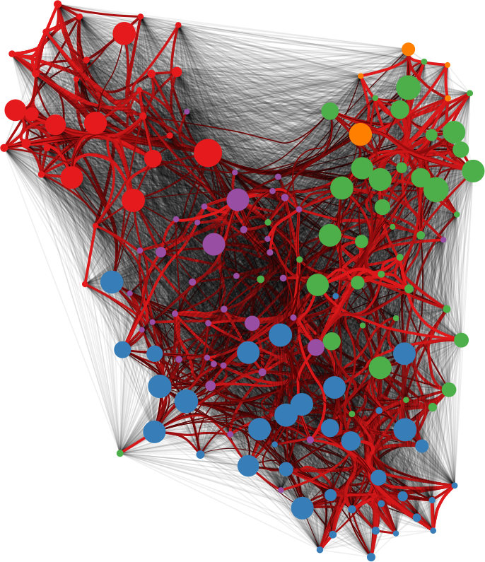
Networks are a fantastic tool for understanding an interconnected world. But, to paraphrase Spider Man, with networks’ expressive power come great headaches. Networks lure us in with their promise of clearly representing complex phenomena. However, once you start working with them, all you get is a tangled mess. This is because, most of the time, there’s noise in the data and/or there are too many connections: you need to weed out the spurious ones. The process of shaving the hairball by keeping only the significant connections — the red ones in the picture below — is called “network backboning”. The network backbone represents the true relationships better and will play much nicer with other network algorithms. In this post, I describe a backboning method I developed with Frank Neffke, from the paper “Network Backboning with Noisy Data” accepted for publication in the International Conference on Data Engineering (the code implementing the most important backbone algorithms is available here).
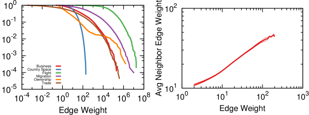
Network backboning is as old as network analysis. The first solution to the problem was to keep edges according to their weight. If you want to connect people who read the same books, pairs who have few books in common are out. Serrano et al. pointed out that edge weight distributions can span many orders of magnitude — as shown in the figure below (left). Even with a small threshold, we are throwing away a lot of edges. This might not seem like a big deal — after all we’re in the business of making the network sparser — except that the weights are not distributed randomly. The weight of an edge is correlated with the weights of the edges sharing a node with it — as shown by the figure below (right). It is easy to see why: if you have a person who read only one book, all its edges can have at most weight one.
Their weights might be low in comparison with the rest of the network, but they are high for their nodes, given their propensity to connect weakly. Isolating too many nodes because we accidentally removed all their edges is a no-no, so Serrano and coauthors developed the Disparity Filter (DF): a technique to estimate the significance of one node’s connections given its typical edge weight, regardless of what the rest of the network says.
This sounds great, but DF and other network backboning approaches make imprecise assumptions about the possibility of noise in our estimate of edge weights. In our book example, noise means that a user might have accidentally said that she read a book she didn’t, maybe because the titles were very similar. One thing DF gets wrong is that, when two nodes are not connected in the raw network data, it would say that measurement error is absent. This is likely incorrect, and it screams for a more accurate estimate of noise. I’m going to leave the gory math details in the paper, but the bottom line is that we used Bayes’ rule. The law allows us to answer the question: how surprising is the weight of this edge, given the weights of the two connected nodes? How much does it defy my expectation?
The expectation here can be thought of as an extraction without replacement, much like Bingo (which statisticians — notorious for being terrible at naming things — would call a “hypergeometric” one). Each reader gets to extract a given number of balls (n, the total number of books she read), drawing from a bin in which all balls are the other users. If a user read ten books, then there are ten balls representing her in the bin. This is a good way to have an expectation for zero edge weights (nodes that are not connected), because we can estimate the probability of never extracting a ball with a particular label.
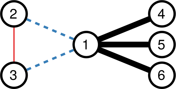
I highlighted the words one and two, because they’re a helpful key to understand the practical difference between the approaches. Consider the toy example below. In it, each edge’s thickness is proportional to its weight. Both DF and our Noise Corrected backbone (NC) select the black edges: they’re thick and important. But they have different opinions about the blue and red edges. DF sees that nodes 2 and 3 have mostly weak connections, meaning their thick connection to node 1 stands out. So, DF keeps the blue edges and it drops the red edge. It only ever looks at one node at a time.
NC takes a different stance. It selects the red edge and drops the blue ones. Why? Because for NC what matters more is the collaboration between the two nodes. Sure, the blue connection is thicker than the red one. But node 1 always has strong connections, and its blue edges are actually particularly weak. On the other hand, node 3 usually has weak connections. Proportionally speaking, the red edge is more important for it, and so it gets saved.
To sum up, NC:
- Refines our estimate of noise in the edge weights;
- Sees an edge as the collaboration between two nodes rather that an event happening to one of them;
- Uses a different model exploiting Bayes’ law to bake these aspects together.
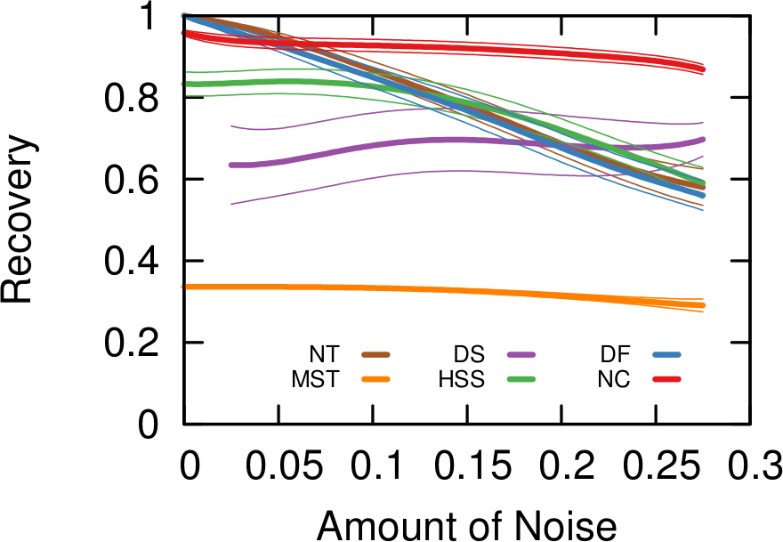
How does that work for us in practice? Above you see some simulations made with artificial networks, of which we know the actual underlying structure, plus some random noise — edges thrown in that shouldn’t exist. The more noise we add the more difficult it is to recover the original structure. When there is little noise, DF (in blue) is better. NC (in red) starts to shine as we increase the amount of noise, because that’s the scenario we were targeting.
In the paper we also show that NC backbones have a comparable stability with DF, meaning that extracting the backbone from different time snapshots of the same phenomenon usually does not yield wildly different results. Coverage — the number of nodes that still have at least one edge in the network — is also comparable. Then we look at quality. When we want to predict some future relationship among the nodes, we expect noisy edges to introduce errors in the estimates. Since a backbone aims at throwing them away, it should increase our predictive power. The table below (click it to enlarge) shows that, in different country-country networks, the predictive quality (R2) using an NC backbone is higher than the one we get using the full noisy network. The quality of prediction can get as high as twice the baseline (the table reports the quality ratio: R2 of the backbone over R2 of the full network, for different methods).
The conclusion is that, when you are confident about the measurement of your network, you should probably extract its backbone using DF. However, in cases of uncertainty, NC is the better option. You can test it yourself!
