25 January 2017 ~ 0 Comments

Network Backboning with Noisy Data

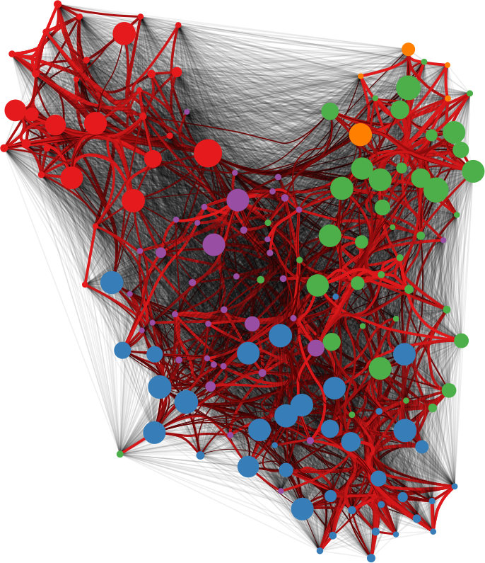
Networks are a fantastic tool for understanding an interconnected world. But, to paraphrase Spider Man, with networks’ expressive power come great headaches. Networks lure us in with their promise of clearly representing complex phenomena. However, once you start working with them, all you get is a tangled mess. This is because, most of the time, there’s noise in the data and/or there are too many connections: you need to weed out the spurious ones. The process of shaving the hairball by keeping only the significant connections — the red ones in the picture below —  is called “network backboning”. The network backbone represents the true relationships better and will play much nicer with other network algorithms. In this post, I describe a backboning method I developed with Frank Neffke, from the paper “Network Backboning with Noisy Data” accepted for publication in the International Conference on Data Engineering (the code implementing the most important backbone algorithms is available here).

bb1

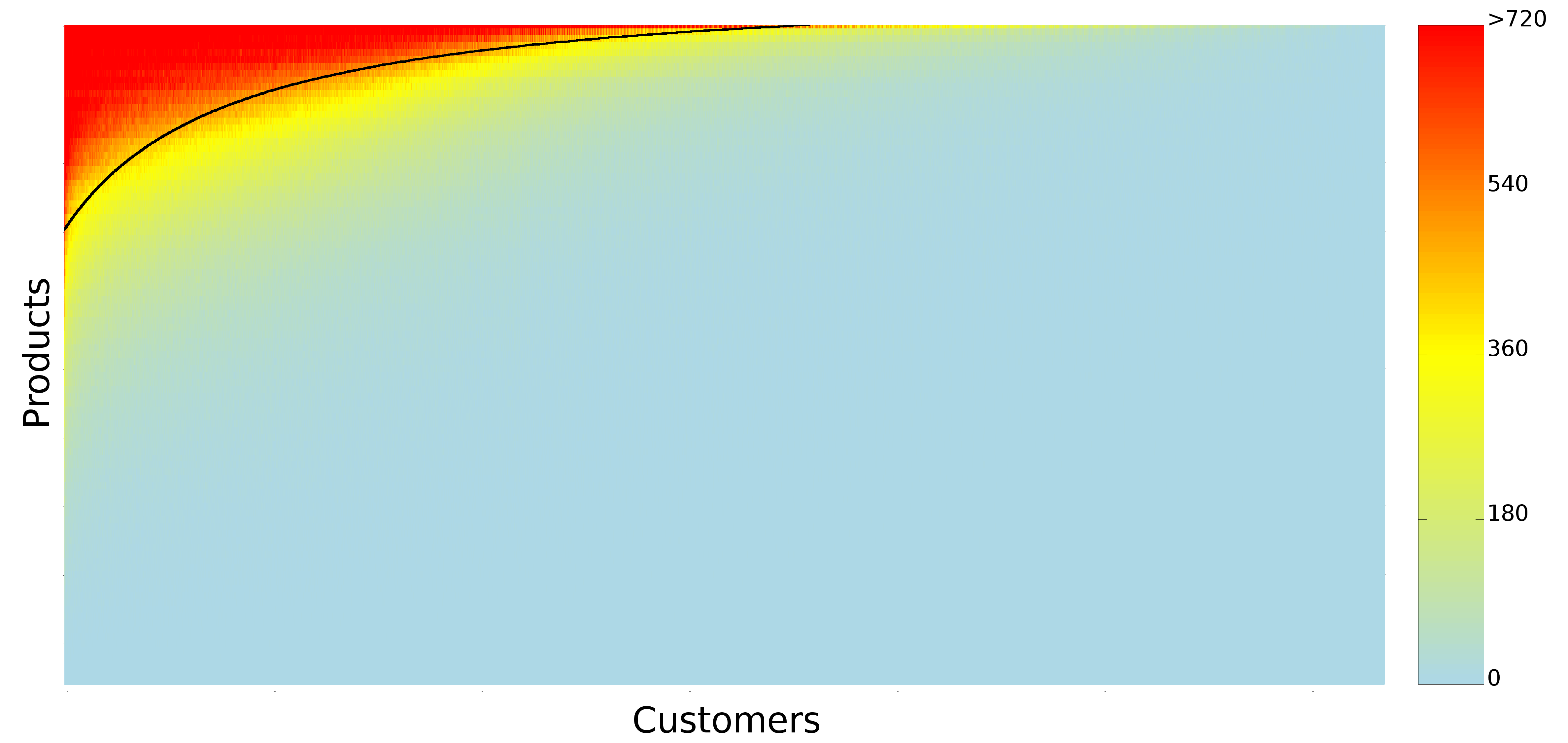
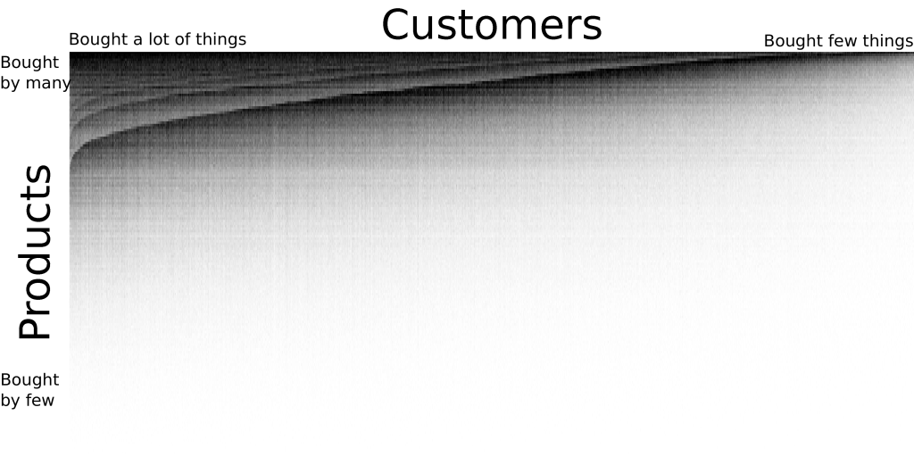
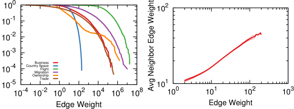
Network backboning is as old as network analysis. The first solution to the problem was to keep edges according to their weight. If you want to connect people who read the same books, pairs who have few books in common are out. Serrano et al. pointed out that edge weight distributions can span many orders of magnitude — as shown in the figure below (left). Even with a small threshold, we are throwing away a lot of edges. This might not seem like a big deal — after all we’re in the business of making the network sparser — except that the weights are not distributed randomly. The weight of an edge is correlated with the weights of the edges sharing a node with it — as shown by the figure below (right). It is easy to see why: if you have a person who read only one book, all its edges can have at most weight one.

Their weights might be low in comparison with the rest of the network, but they are high for their nodes, given their propensity to connect weakly. Isolating too many nodes because we accidentally removed all their edges is a no-no, so Serrano and coauthors developed the Disparity Filter (DF): a technique to estimate the significance of one node’s connections given its typical edge weight, regardless of what the rest of the network says.

bb2

This sounds great, but DF and other network backboning approaches make imprecise assumptions about the possibility of noise in our estimate of edge weights. In our book example, noise means that a user might have accidentally said that she read a book she didn’t, maybe because the titles were very similar. One thing DF gets wrong is that, when two nodes are not connected in the raw network data, it would say that measurement error is absent. This is likely incorrect, and it screams for a more accurate estimate of noise. I’m going to leave the gory math details in the paper, but the bottom line is that we used Bayes’ rule. The law allows us to answer the question: how surprising is the weight of this edge, given the weights of the two connected nodes? How much does it defy my expectation?

The expectation here can be thought of as an extraction without replacement, much like Bingo (which statisticians — notorious for being terrible at naming things — would call a “hypergeometric” one). Each reader gets to extract a given number of balls (n, the total number of books she read), drawing from a bin in which all balls are the other users. If a user read ten books, then there are ten balls representing her in the bin. This is a good way to have an expectation for zero edge weights (nodes that are not connected), because we can estimate the probability of never extracting a ball with a particular label.

bb4

I highlighted the words one and two, because they’re a helpful key to understand the practical difference between the approaches. Consider the toy example below. In it, each edge’s thickness is proportional to its weight. Both DF and our Noise Corrected backbone (NC) select the black edges: they’re thick and important. But they have different opinions about the blue and red edges. DF sees that nodes 2 and 3 have mostly weak connections, meaning their thick connection to node 1 stands out. So, DF keeps the blue edges and it drops the red edge. It only ever looks at one node at a time.

bb5

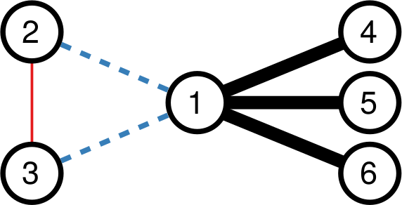
NC takes a different stance. It selects the red edge and drops the blue ones. Why? Because for NC what matters more is the collaboration between the two nodes. Sure, the blue connection is thicker than the red one. But node 1 always has strong connections, and its blue edges are actually particularly weak. On the other hand, node 3 usually has weak connections. Proportionally speaking, the red edge is more important for it, and so it gets saved.

To sum up, NC:

  1. Refines our estimate of noise in the edge weights;
  2. Sees an edge as the collaboration between two nodes rather that an event happening to one of them;
  3. Uses a different model exploiting Bayes’ law to bake these aspects together.

bb6

How does that work for us in practice? Above you see some simulations made with artificial networks, of which we know the actual underlying structure, plus some random noise — edges thrown in that shouldn’t exist. The more noise we add the more difficult it is to recover the original structure. When there is little noise, DF (in blue) is better. NC (in red) starts to shine as we increase the amount of noise, because that’s the scenario we were targeting.

In the paper we also show that NC backbones have a comparable stability with DF, meaning that extracting the backbone from different time snapshots of the same phenomenon usually does not yield wildly different results. Coverage — the number of nodes that still have at least one edge in the network — is also comparable. Then we look at quality. When we want to predict some future relationship among the nodes, we expect noisy edges to introduce errors in the estimates. Since a backbone aims at throwing them away, it should increase our predictive power. The table below (click it to enlarge) shows that, in different country-country networks, the predictive quality (R2) using an NC backbone is higher than the one we get using the full noisy network. The quality of prediction can get as high as twice the baseline (the table reports the quality ratio: R2 of the backbone over R2 of the full network, for different methods).

bb8

The conclusion is that, when you are confident about the measurement of your network, you should probably extract its backbone using DF. However, in cases of uncertainty, NC is the better option. You can test it yourself!

Continue Reading

18 December 2014 ~ 0 Comments

The Supermarket is an Ecosystem

There are few things that you would consider less interesting than doing groceries at the supermarket. For some it’s a chore, others probably like it. But for sure you don’t see much of a meaning behind it. It’s not that you sense around you a grave atmosphere, the kind of mysterious background radiance you perceive when you feel part of Something Bigger. Just buy the bloody noodles already. Well, to some extent you are wrong.

Of course the reality is less mystical than what I tried to led you to believe in this opening paragraph. But it turns out that customers of a supermarket chain behave as if they were playing a specific role. These roles are the focus of the paper I recently authored with Diego Pennacchioli, Salvatore Rinzivillo, Dino Pedreschi and Fosca Giannotti. It has been published on the journal EPJ Data Science, and you can read it for free.

So what are these roles? The title of the paper is very telling: the retail market is a complex system. So the first thing to clear out is what the heck a complex system is. This is not so easily explained – otherwise it wouldn’t be complex, duh. The precise physics definition of complex systems might be too sophisticated. For this post, it will be sufficient to use the following one: a complex system is a collection of interacting parts and its behavior cannot be expressed as a sum of the behaviors of its parts. A good example of complexity is Earth’s ecosystem: there are so many interacting animals and phenomena that having a perfect description of it by just listing all interactions is just impossible.

lake-ecosystem-1_438x0_scale

And a supermarket is basically the same. In the paper we propose several proofs of it, but the one that goes best with the chosen example involves the esoteric word “nestedness”. When studying different ecosystems, some smart dudes decided to record their observations in matrix form. For each different island (ecosystem) they recorded if a particular species was present or not. When they looked at the resulting matrix they noticed a particular pattern. The islands with few species had only the species that were found in all islands, and at the same time the most rare species were present exclusively in those islands which were hosting all the observed species. If you reordered the islands by species count and the species by island count, the matrix had a particular triangular shape. They called matrices like that “nested”.

We did the same thing with customers and products. There are customers who buy only a handful of products: milk, water, bread. And those products are the products that everybody buys. Then there are those customers who, over a year, buy basically everything you can see in a supermarket. And they are the only ones buying the least sold products. The customers X products matrix ends up looking exactly like an ecosystem nested matrix (you probably already saw it over a year ago on this blog – in fact, this work builds on the one I wrote about back then, but the matrix picture is much prettier, thanks to Diego Pennacchioli):

matrix

Since we have too many products and customers, this is a compressed view and the color tells you how many observations we have per pixel (click for full resolution). One observation is simply a pairing of a customer and a product, indicating that the customer bought that product in significant quantities over a year. Ok, where does this bring us? First, as parts of a complex system, customers are not so easily classifiable. Marketing is all about finding uniformly behaving groups of people. The consequence of being complex parts is that this task is hopeless. You cannot really put people into bins. People are part of a continuous space, as shown in the picture, and every cut-off you propose is necessarily arbitrary.

The solution to this problem is represented by that black line you see on the matrix. That line is trying to divide the matrix in two parts: a part where we mostly have ones, and a part where we mostly have zeroes. The line does not match reality perfectly. It is a hyperbola that we told to fit itself as snugly to the data as possible. Once estimated, the function of the black line enables a neat application: to predict the next product a customer is interested in buying.

Remember that the matrix has its columns and rows sorted. The first customer is the one who bought the most products, the second bought a little less product and so on with increasing ranks. Same thing with products: the highest ranked (1st) is sold to most customers, the lowest ranked is sold to just one customer. This means that if you have the black line formula and the rank of a customer, you can calculate the rank of a corresponding product. Given that the black line divides the ones from the zeros, this product is a zero that can most easily become a one or, in other words, the supermarket’s best bet of what product the customer is most likely to want to buy next. You do not need customer segmentation any more: since the matrix is and will always be nested you just have to fill it following the nested pattern, and the black line is your roadmap.

pyramid

We can use the ranks of the products for a description of customer’s needs. The highest ranked products are bought by everyone, so they are satisfying basic needs.  We decided to depict this concept borrowing Maslow’s pyramid of needs. The one reported above is interesting (again, click for full resolution), although it applies only to the supermarket area our data is coming from. In any case it is interesting how some things that are on the basis of Maslow’s pyramid are on top of our, for example having a baby. You could argue that many people do not buy those products in a supermarket, but we address these concerns in the paper.

So next time you are pondering whether buying or not buying that box of six donuts remember: you are part of a gigantic system and the little weight you might gain is insignificant compared to the beautiful role you are playing. So go for it, eat the hell out of those bad boys.

Continue Reading

09 September 2013 ~ 0 Comments

What Motivates a Customer

The Holy Grail of every marketing system is to understand how the mind of the customers works. For example answering the question: “From how far can I attract customers?” To do so means to increase profits. You can deploy your communication and products more efficiently and maximize your returns. Clearly, there is no silver bullet for this task. There is no way that one single aspect is so predominant in a person’s mind at the point of empowering a seller to have perfect control over who will buy her product, where and when. If that would be true, there would be no space left for marketing specialists, demand segmentation and so on. Many little tricks can be deployed in the market.

I am by no means an expert on the field, so my way to frame this problem may sound trivial. In any case, I can list three obvious parameters that affect a customer’s decision in buying or not buying a product. The first is price. Few people want to throw their money senselessly, most of them want to literally maximize the bang for their buck (okay, maybe not that literally). The second is the quantities needed: if I need to buy product X everyday in large bulks and product Y once in a blue moon, then it’s only fair to assume that I’ll consider different parameters to evaluate X and Y.

question

The third is the level of sophistication of a given product. There are things that fewer and fewer people need: birdseed, piña colada flavored lip balm. Narrower customer base means less widespread offer, thus the need of travel more to specialized shops. Intuitively, sophistication is more powerful than price and quantity: a Lamborghini is still a car – also quite useless when doing groceries – like a Panda, but it satisfies very different and much more sophisticated needs. Sophistication is powerful because you can play with it, increasing the perceived sophistication of a product, thus your market: like Jonah Berger‘s  “thee types of ice” bar, that looked more fancy just by inventing a way to make ice sound more sophisticated than it is.

So let’s play and try to use these concepts operatively. Say we want to predict the distance a customer is willing to travel to buy a product. Then, we try to predict such a distance using different variables. The one leading to better predictions of these distances wins as the best variable describing what motivates a customer to travel. We decided to test the three variables I presented before: price, quantity and sophistication. In this theory, higher prices mean longer distances to travel, as if I have to buy an expensive TV I’ll probably go around and check where is the best quality-price ratio. Higher quantities mean shorter distances, as if I have to buy bread everyday I don’t care where the best bakery of the city is if that means traveling ten kilometers everyday. Finally, higher sophistication means longer distances: if I have sophisticated needs I need to travel a lot to satisfy them.

Price and quantity are easy to deal with: they are just numbers. So we can put them on the X axis of a plot and put the distance traveled on the Y axis. And that’s what we did, for price:

scatter1

and for quantity:

scatter2

Here, each dot is a customer buying a product. If the dots had the same distance and the same price/quantity then we merged them together (brighter color = more dots here). We see that our theory, while not perfect, is correct: higher prices means longer distances traveled, higher quantities means shorter distances. Time to test for the level of sophistication! But now we hit a brick wall. How on earth am I suppose to measure the level of sophistication of a person and of a product? Should I split the brain of that person in half? How can I do this for thousands or millions of customers? We need to invent a brain splitting machine.

inside-the-customers-mind1

That’s more or less what we did. In a joint work with Diego Pennacchioli, Salvo Rinzivillo, Fosca Giannotti and Dino Pedreschi, that will appear in the BigData 2013 conference (you can download the paper, if you are interested), we proposed such a brain slice device. Of course I am somewhat scared by all the blood that would result in literally cutting open thousands of skulls, so we implemented a data mining machine that just quantifies with a number the level of sophistication of a customer’s needs and the level of sophistication that a product can satisfy, solving the issue at hand with no bloodshed.

The fundamental question is: is the level of sophistication a number? Intuition would tell us “no”: it’s a complex multidimensional space and my needs are unique like a snowflake. Kind of. But with a satisfying level of approximation, surprisingly, we can describe sophistication with a number. How is that possible? A couple of facts we discovered: customers buying the least sold products also buy everything else (the “simpler” stuff), and products bought just by few customers are bought only by those who also buy everything else. In other words, if you draw a matrix connecting the customers with the products they buy, this matrix is nested, meaning that all purchases are in the top left corner:

matrix

A-ha! Then it’s fair to make this assumption: customers are adding an extra product bought only if they already buy (almost) everything else “before” it. This implies two things: first, is that they add the extra product if all their previous products already satisfied their more basic needs (then, they are more sophisticated); second, is that they are moving on a monodimensional space, adding stuff incrementally. Then, they can be quantified by a number! I won’t go in the boring details about how to calculate this number. Suffice to say that they are very similar to how you calculate a country’s complexity, about which I wrote months ago; and that this number is not the total amount of money they spend, nor the quantity of products they buy.

So, how does this number relate to the distance traveled by customers?

scatter3

The words you are looking for is “astonishingly well”.

So our quantification of the sophistication level has a number of practical applications. In the paper we explore the task of predicting in which shop a customers will go to buy a given product. We are not claiming that this is the only important factor. But it gives a nice boost. Over a base accuracy of around 53%, using the price or the quantity gives you a +6-7% accuracy. Adding the sophistication level gives an additional +6-8% accuracy (plots would suggest more, but they are about continuous numbers, while in reality shop position is fixed and therefore a mistake of a few hundreds meters is less important). Not bad!

Continue Reading