The Curious World of Network Mapping
Complex networks can come in different flavors. As you know if you follow this blog, my signature dish is multilayer/multidimensional networks: networks with multiple edge types. One of the most popular types is bipartite networks. In bipartite networks, you have two types of nodes. For example, you can connect users of Netflix to the movies they like. As you can see from this example, in bipartite networks we allow only edges going from one type of nodes to the other. Users connect to movies, but not to other users, and movies can’t like other movies (movies are notoriously mean to each other).

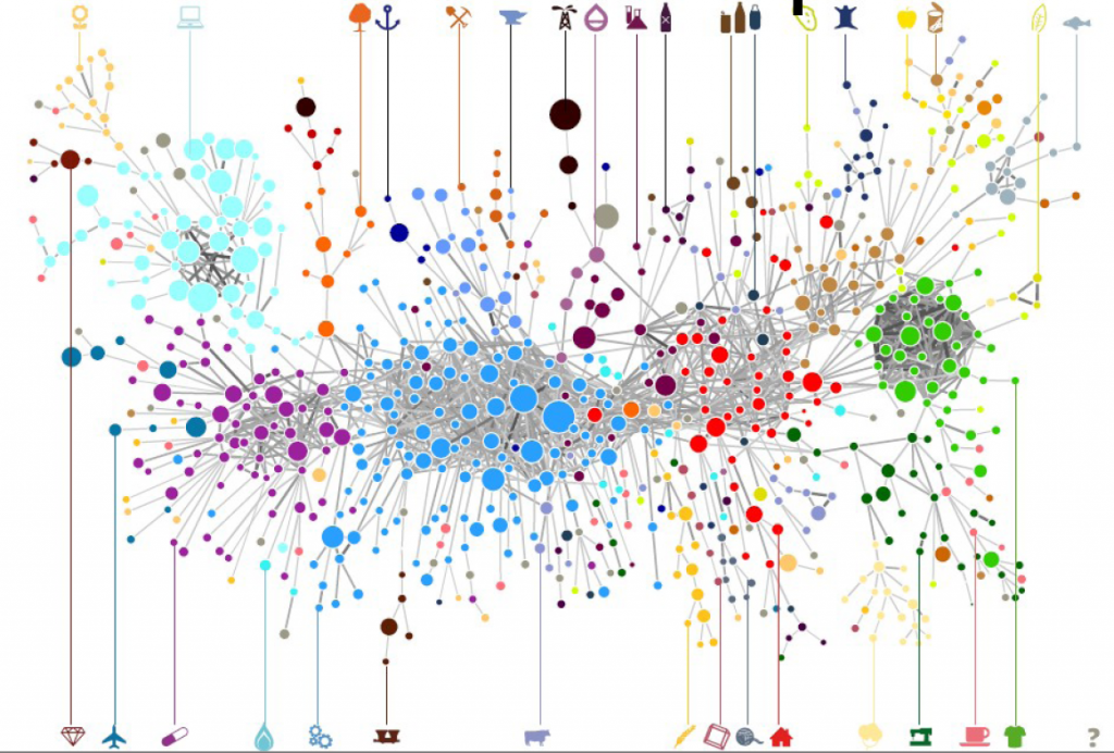
Many things (arguably almost everything) can be represented as a bipartite network. An occupation can be connected to the skills and/or tasks it requires, an aid organization can be connected to the countries and/or the topics into which it is interested, a politician is connected to the bills she sponsored. Any object has attributes. And so it can be represented as an object-attribute bipartite network. However, most of the times you just want to know how similar two nodes of the same type are. For example, given a movie you like, you want to know a similar movie you might like too. This is called link prediction and there are two ways to do this. You could focus on predicting a new user-movie connection, or focus instead on projecting the bipartite network to discover the previously unknown movie-movie connections. The latter is the path I chose, and the result is called “Network Map”.
It is clearly the wrong choice, as the real money lies in tackling the former challenge. But if I wanted to get rich I wouldn’t have chosen a life in academia anyway. The network map, in fact, has several advantages over just predicting the bipartite connections. By creating a network map you can have a systemic view of the similarities between entities. The Product Space, the Diseasome, my work on international aid. These are all examples of network maps, where we go from a bipartite network to a unipartite network that is much easier to understand for humans and to analyze for computers.

Creating a network map, meaning going from a user-movie bipartite network to a movie-movie unipartite network, is conceptually easy. After all, we are basically dealing with objects with attributes. You just calculate a similarity between these attributes and you are done. There are many similarities you can use: Jaccard, Pearson, Cosine, Euclidean distances… the possibilities are endless. So, are we good? Not quite. In a paper that was recently accepted in PLoS One, Muhammed Yildirim and I showed that real world networks have properties that make the general application of any of these measures quite troublesome.
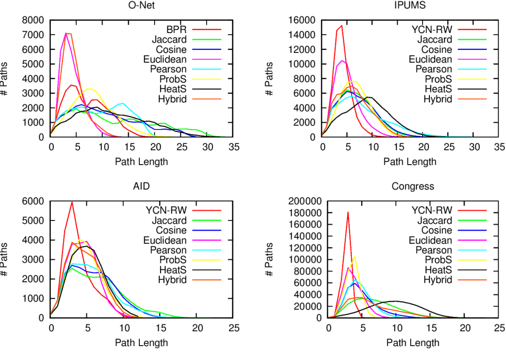
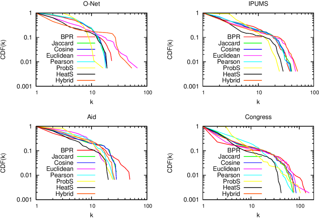
For example, bipartite networks have power-law degree distributions. That means that a handful of attributes are very popular. It also means that most objects have very few attributes. You put the two together and, with almost 100% probability, the many objects with few attributes will have the most popular attributes. This causes a great deal of problems. Most statistical techniques aren’t ready for this scenario. Thus they tend to clutter the network map, because they think that everything is similar to everything else. The resulting network maps are quite useless, made of poorly connected dense areas and lacking properties of real world networks, such as power-law degree distributions and short average path length, as shown in these plots:


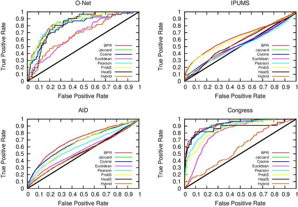
Of course sometimes some measure gets it right. But if you look closely at the pictures above, the only method that consistently give the shortest paths (above, when the peak is on the left we are good) and the broadest degree distributions (below, the rightmost line at the end in the lower-right part of the plot is the best one) is the red line of “BPR”. BPR stands for “Bipartite Projection via Random-walks” and it happens to be the methodology that Muhammed and I invented. BPR is cool not only because its network maps are pretty. It is also achieving higher scores when using the network maps to predict the similarity between objects using ground truth, meaning that it gives the results we expect when we actually already know the answers, that are made artificially invisible to test the methodology. Here we have the ROC plots, where the highest line is the winner:

So what makes BPR so special? It all comes down to the way you discount the popular attributes. BPR does it in a “network intelligent” way. We unleash countless random walkers on the bipartite network. A random walker is just a process that starts from a random object of the network and then it jumps from it to one of its attributes. The target attribute is chosen at random. And then the walker jumps back to an object possessing that attribute, again choosing it at random. And then we go on. At some point, we start from scratch with a new random walk. We note down how many times two objects end up in the same random walk and that’s our similarity measure. Why does it work? Because when the walker jumps back from a very popular attribute, it could essentially go to any object of the network. This simple fact makes the contribution of the very popular attributes quite low.
BPR is just the latest proof that random walks are one of the most powerful tools in network analysis. They solve node ranking, community discovery, link prediction and now also network mapping. Sometimes I think that all of network science is founded on just one algorithm, and that’s random walks. As a final note, I point out that you can create your own network maps using BPR. I put the code online (the page still bears the old algorithm’s name, YCN). That’s because I am a generous coder.
