08 March 2023 ~ 0 Comments

Quantifying Ideological Polarization on Social Media

Ideological polarization is the tendency of people to hold more extreme political opinions over time while being isolated from opposing points of view. It is not a situation we would like to get out of hand in our society: if people adopt mutually incompatible worldviews and cannot have a dialogue with those who disagree with them, bad things might happen — violence, for instance. Common wisdom among scientists and laymen alike is that, at least in the US, polarization is on the rise and social media is to blame. There’s a problem with this stance, though: we don’t really have a good measure to quantify ideological polarization.

This motivated Marilena Hohmann and Karel Devriendt to write a paper with me to provide such a measure. The result is “Quantifying ideological polarization on a network using generalized Euclidean distance,” which appeared on Science Advances earlier this month.
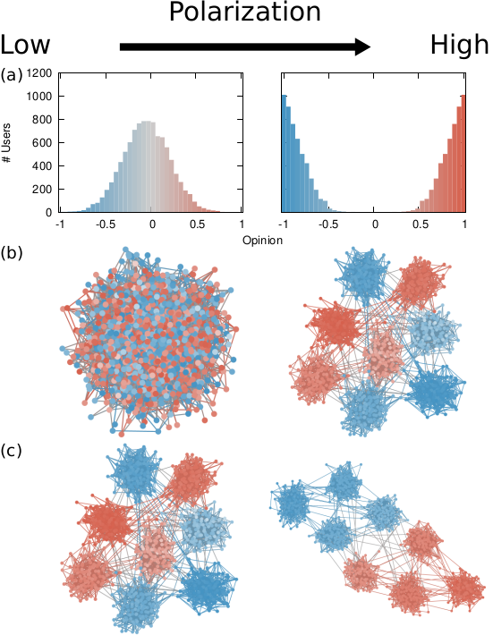
The components of our polarization definition, from top to bottom: (a) ideology, (b) dialogue, and (c) ideology-dialogue interplay. The color hue shows the opinion of a node, and its intensity is how strongly the opinion is held.

Our starting point was to stare really hard at the definition of ideological polarization I provided at the beginning of this post. The definition has two parts: stronger separation between opinions held by people and lower level of dialogue between them. If we look at the picture above we can see how these two parts might look. In the first row (a) we show how to quantify a divergence of opinion. Suppose each of us has an opinion from -1 (maximally liberal) to +1 (maximally conservative). The more people cluster in the middle the less polarization there is. But if everyone is at -1 or +1, then we’re in trouble.

The dialogue between parts can be represented as a network (second row, b). A network with no echo chambers has a high level of dialogue. As soon as communities of uniform opinions arise, it is more difficult for a person of a given opinion to hear the other side. This dialogue is doubly difficult if the communities themselves organize in the network as larger echo chambers (third row, c): if all communities talk to each other we have less polarization than if communities only engage with other communities that hold more similar opinions.
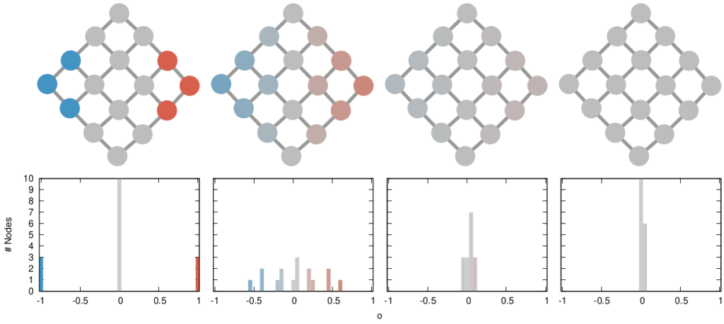
In this image, time flows from left to right: the first column is the initial condition with the node color proportional to its temperature, then we let heat flow through the edges. The plot on the second row shows the temperature distribution of the nodes.

The way we decided to approach the problem was to rely on the dark art spells of Karel, the Linear Algebra Wizard to simulate the process of opinion spreading. In practice, you can think the opinion value of each person to be a certain temperature, as the image above shows. Heat can flow through the connections of the network: if two nodes are at different temperatures they can exchange some heat per unit of time, until they reach an equilibrium. Eventually all nodes converge to the average temperature of the network and no heat can flow any longer.

The amount of time it takes to reach equilibrium is the level of polarization of the network. If we start from more similar opinions and no communities, it takes little to converge because there is no big temperature difference and heat can flow freely. If we have homogeneous communities at very different temperature levels it takes a lot to converge, because only a little heat can flow through the sparse connections between these groups. What I describe is a measure called “generalized Euclidean distance”, something I already wrote about.
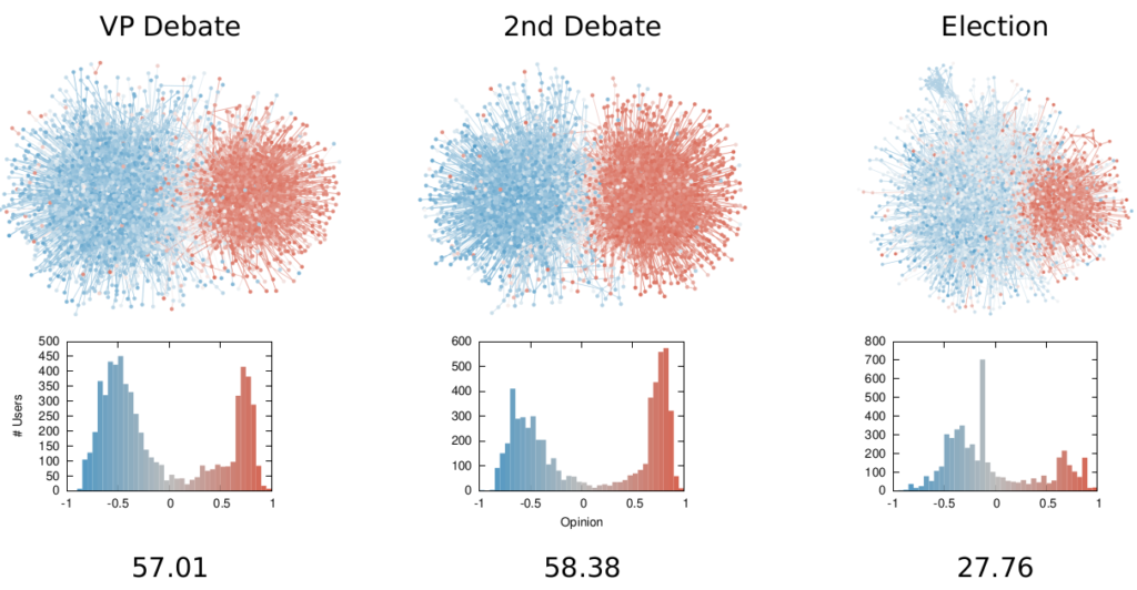
Each node is a Twitter user reacting to debates and the election night. Networks on the top row, opinion distributions in the middle, polarization values at the bottom.

There are many measures scientists have used to quantify polarization. Approaches range from calculating homophily — the tendency of people to connect to the individuals who are most similar to them –, to using random walks, to simulating the spread of opinions as if they were infectious diseases. We find that all methods used so far are blind and/or insensitive to at least one of the parts of the definition of ideological polarization. We did… a lot of tests. The details are in the paper and I will skip them here so as not to transform this blog post into a snoozefest.

Once we were happy with a measure of ideological polarization, we could put it to work. The image above shows the levels of polarization on Twitter during the 2020 US presidential election. We can see that during the debates we had pretty high levels of polarization, with extreme opinions and clear communities. Election night was a bit calmer, due to the fact that a lot of users engaged with the factual information put out by the Associated Press about the results as they were coming out.
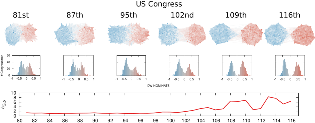
Each node is a congressman. One network per US Congress in the top row, DW-NOMINATE scores distributions in the middle row, and timeline of polarization levels in the bottom.

We are not limited to social media: we can apply our method to any scenario in which we can record the opinions of a set of people and their interactions. The image above shows the result for the US House of Representatives. Over time, congresspeople have drifted farther away in ideology and started voting across party lines less and less. The network connects two congresspeople if they co-voted on the same bill a significant number of times. The most polarized House in US history (until the 116th Congress) was the 113th, characterized by a debt-ceiling crisis following the full application of the Affordable Care Act (Obamacare), the 2014 Russo-Ukrainian conflict, strong debates about immigration reforms, and a controversial escalation of US military action in Syria and Iraq against ISIS.

Of course, our approach has its limitations. In general, it is difficult to compare two polarization scores from two systems if the networks are not built in the same way and the opinions are estimated using different measures. For instance, in our work, we cannot say that Twitter is more polarized than the US Congress (even though it has higher scores), because the edges represent different types of relations (interacting on Twitter vs co-voting on a bill) and the measures of opinions are different.

We feel that having this measure is a step in the right direction, because at least it is more accurate than anything we had so far. All the data and code necessary to verify our claims is available. Most importantly, the method to estimate ideological polarization is included. This means you can use it on your own networks to quantify just how fu**ed we are the healthiness of our current political debates.
Continue Reading

15 April 2021 ~ 0 Comments

A Bayesian Framework for Online Social Network Sampling

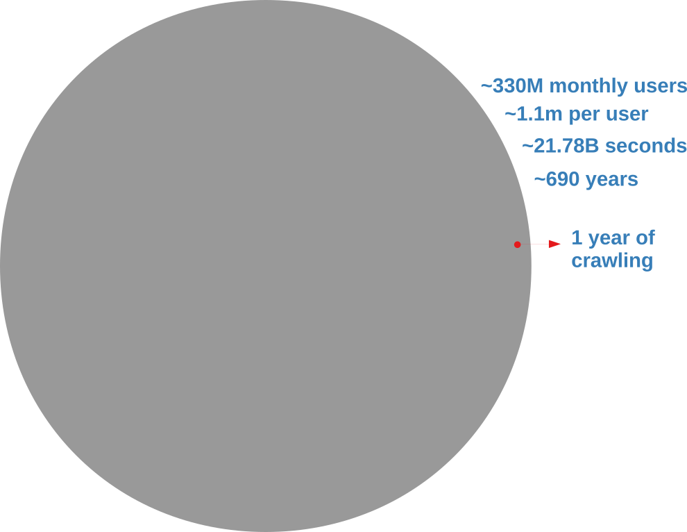
Analyzing an online social network is hard because there’s no “download” button to get the data. In the best case scenario, you have to query an API (Application Program Interface) system. You have to tell the API which user you want to see the connections of, and you can’t just ask for all users at the same time. With the current API rate limits, downloading the Twitter graph would take seven centuries, as the picture below explains.

The gray circle represents the totality of Twitter’s users. The red one is what you’d get with a continuous crawl of one year.

I don’t know about you, but I don’t have seven centuries to publish my papers. I want to become a famous scientist now. If you’re like me, you’re forced to extract only a sample. In this post, I’ll describe a network sampling algorithm that works with social media APIs to maximize the amount of information you get from your sample. The method has been published in the paper “Noise Corrected Sampling of Online Social Networks“, which recently appeared in the journal Transactions on Knowledge Discovery from Data.

My Noise Corrected sampling (NC) is a topological method. This means that you start from one (or more) user IDs that are known, and then you gather new user IDs from their friends, then you move on to the friends’ friends and so on, following the connections in the graph you’re sampling. This is the usual approach, because there is no way to know the user IDs beforehand — unless you have inside knowledge about how the social media platform works.

The underlying common question behind a topological sampler is: how do we pick the best user to explore next? Different samplers answer this question differently. A Random Walk sampler says: “Screw it! Thinking is too hard! I’m gonna get a random node from the friends of the currently explored node! Then, with the time I saved, I’m gonna get some ice cream.” The Metropolis-Hastings Random Walk — the nerd’s answer to the jock’s Random Walk — wants to preserve the degree distribution, so it penalizes high-degree nodes — since they’re more likely to be oversampled. Alternatively, we could use classical graph exploration techniques such as Depth-First and Breadth-First Search — and, again, you can enhance them so that you can preserve some properties of the network, for instance its clustering coefficient.

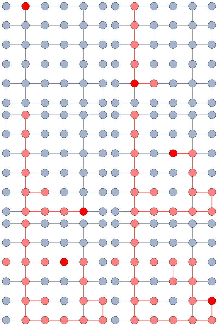
A random walk on a graph. It looks like a drunk going around. I don’t drink and sample, and neither should you.

My NC departs from all these approaches in a fundamental way. The thing they all have in common is that they don’t use information from the sample they have currently gathered. They only look at the potential next users and make a decision on whom to explore based on their characteristics alone. For instance Metropolis-Hastings Random Walk checks the user’s popularity in number of connections. NC, instead, looks at the entire collected sample and asks a straightforward question: “which of these next users is most likely to give me the most information about the whole structure, given what I explored so far?”

It does so with a Bayesian framework. The gory math is in the paper, but the underlying philosophy is that you can calculate a z-score for each edge of the network. It tells you how surprising it is that this edge is there. In probability theory, “surprise” is a good thing: it is directly related to how much information something gives you. Probability theorists are a bunch of jolly folks, always happy to discover jacks-in-a-box. If you always pick the most surprising edge in the network to explore the next user, you’re maximizing the amount of information you’re going to get back. The picture below unravels what this entails on a simple example.

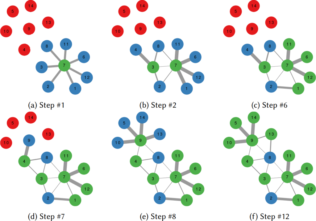
In this example, the green nodes are explored, the blue nodes are known — because they’re friends of an explored node — but not explored yet. The red nodes are unknown.

The first figure (a) is the start of the process, where we have a network and we pick a random starting point, node 7. I use the edge thickness to show its z-score: we always follow the widest edge. Initially, you only pick a random edge, because all edges have the same z-score in a star. However, once I pick node 3, all z-scores change as we discover new edges (b). In this case, first we prioritize the star around node 7 (c), then we start following the path from node 3 until node 9 (d-e), then we explore the star around node 9 until there are no more nodes nor edges to discover in this toy network (f). Note how edges exhaust their surprise as you learn more about the neighborhoods of the nodes they connect.

Our toy example is an unweighted network, where all edges have the same weight, but this method thrives if you have information about how strong a connection is. The edge weight is additional information that can be taken into account to measure its surprise value. Under the hood, NC estimates the expected weight of an edge given the average edge weights of the two nodes it connects. In an unweighted network this is equivalent to the degree, because all edges have the same weight. But in a weighted network you actually have meaningful differences between nodes that tend to have strong/weak connections.

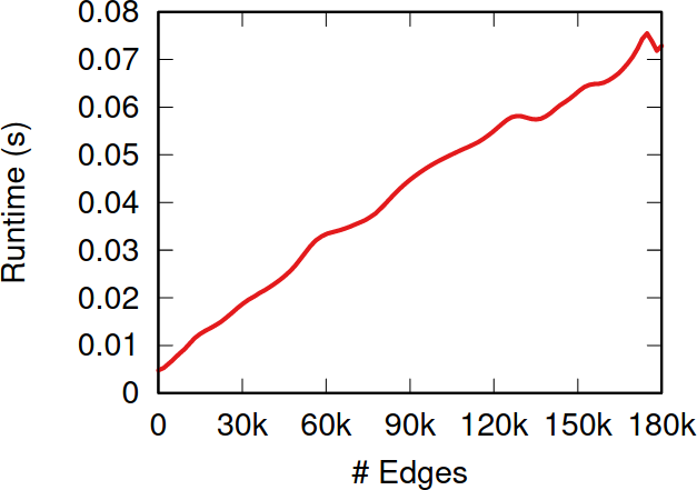
So, the million dollar question: how does NC fare when tested against the alternatives I presented before? The first worry you might have is that it takes too much time to calculate the z-scores. After all, to do so you need to look at the entire sampled network so far, while the other methods only look at a local neighborhood. NC is indeed slower than them—it has to be. But it doesn’t matter. The figure above shows how much time it takes to calculate the z-scores for more and more edges. Those runtimes (less than a tenth of a second) are puny when compared to the multi-second wait times due to the APIs’ rate limits — or even to simple network latency. After all, NC is a simplification of the Noise-Corrected Backbone algorithm I developed with Frank Neffke, and we showed in the original paper that it was pretty darn fast.

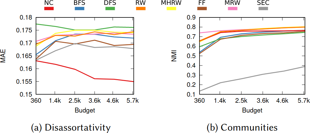
What about the quality of the samples? This is a question with a million answers, because it depends on what you want to do with the sample, besides what are the characteristics of the original graph and of the API system you’re wrestling against, and how much time you have to gather your sample. For instance, in the figure below we see that NC is the best method when you want to estimate the assortativity value of a disassortative attribute (think gender in a dating network), but it is a boring middle-of-the-pack method when you want to reconstruct the original communities of a network.

Left: the Mean Absolute Error between the sample’s and the original graph’s assortativity values (lower is better). Right: the Normalized Mutual Information between the sample’s and the original graph’s communities (higher is better). NC in red.

NC ranks between the 3rd and 4th position on average across a wide range of applications, network topologies, API systems, and budget levels. This is good because I test eight alternatives, thus the expectation is that NC will practically always be better than average. Among all eight methods tested, in fact, no other method has a better rank average. The second best method is Depth-First Search, which ranks 4th three out of four times, against NC’s one out of two.

I have shared some code allowing to replicate my results. If you speak Python better than you speak academiquese, you could use that code to infer how to implement an NC sampling strategy next time you need to download Twitter.

Continue Reading

28 August 2014 ~ 0 Comments

The Curious World of Network Mapping

Complex networks can come in different flavors. As you know if you follow this blog, my signature dish is multilayer/multidimensional networks: networks with multiple edge types. One of the most popular types is bipartite networks. In bipartite networks, you have two types of nodes. For example, you can connect users of Netflix to the movies they like. As you can see from this example, in bipartite networks we allow only edges going from one type of nodes to the other. Users connect to movies, but not to other users, and movies can’t like other movies (movies are notoriously mean to each other).

m1

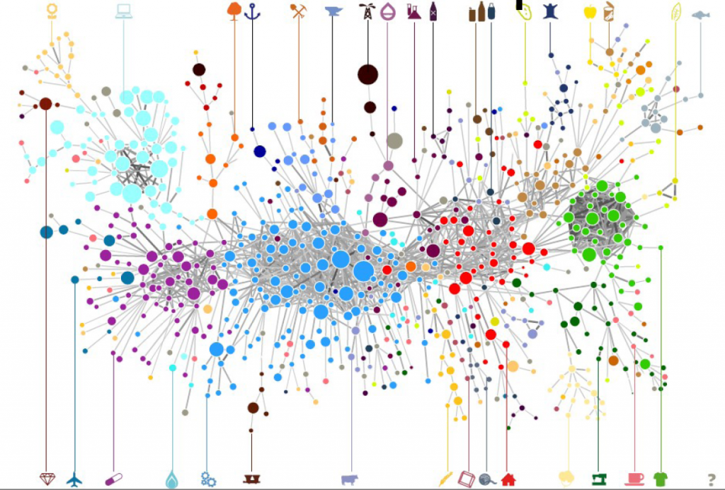
Many things (arguably almost everything) can be represented as a bipartite network. An occupation can be connected to the skills and/or tasks it requires, an aid organization can be connected to the countries and/or the topics into which it is interested, a politician is connected to the bills she sponsored. Any object has attributes. And so it can be represented as an object-attribute bipartite network. However, most of the times you just want to know how similar two nodes of the same type are. For example, given a movie you like, you want to know a similar movie you might like too. This is called link prediction and there are two ways to do this. You could focus on predicting a new user-movie connection, or focus instead on projecting the bipartite network to discover the previously unknown movie-movie connections. The latter is the path I chose, and the result is called “Network Map”.

It is clearly the wrong choice, as the real money lies in tackling the former challenge. But if I wanted to get rich I wouldn’t have chosen a life in academia anyway. The network map, in fact, has several advantages over just predicting the bipartite connections. By creating a network map you can have a systemic view of the similarities between entities. The Product Space, the Diseasome, my work on international aid. These are all examples of network maps, where we go from a bipartite network to a unipartite network that is much easier to understand for humans and to analyze for computers.

ps4

Creating a network map, meaning going from a user-movie bipartite network to a movie-movie unipartite network, is conceptually easy. After all, we are basically dealing with objects with attributes. You just calculate a similarity between these attributes and you are done. There are many similarities you can use: Jaccard, Pearson, Cosine, Euclidean distances… the possibilities are endless. So, are we good? Not quite. In a paper that was recently accepted in PLoS One, Muhammed Yildirim and I showed that real world networks have properties that make the general application of any of these measures quite troublesome.

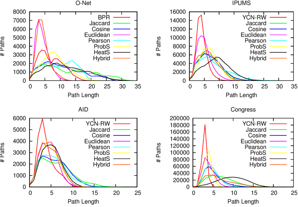
For example, bipartite networks have power-law degree distributions. That means that a handful of attributes are very popular. It also means that most objects have very few attributes. You put the two together and, with almost 100% probability, the many objects with few attributes will have the most popular attributes. This causes a great deal of problems. Most statistical techniques aren’t ready for this scenario. Thus they tend to clutter the network map, because they think that everything is similar to everything else. The resulting network maps are quite useless, made of poorly connected dense areas and lacking properties of real world networks, such as power-law degree distributions and short average path length, as shown in these plots:

m2

m3

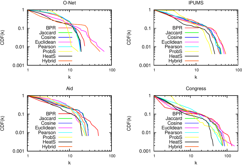
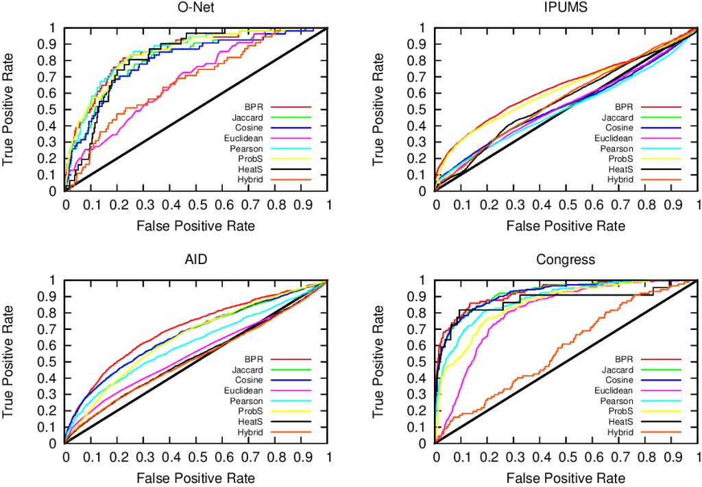
Of course sometimes some measure gets it right. But if you look closely at the pictures above, the only method that consistently give the shortest paths (above, when the peak is on the left we are good) and the broadest degree distributions (below, the rightmost line at the end in the lower-right part of the plot is the best one) is the red line of “BPR”. BPR stands for “Bipartite Projection via Random-walks” and it happens to be the methodology that Muhammed and I invented. BPR is cool not only because its network maps are pretty. It is also achieving higher scores when using the network maps to predict the similarity between objects using ground truth, meaning that it gives the results we expect when we actually already know the answers, that are made artificially invisible to test the methodology. Here we have the ROC plots, where the highest line is the winner:

m4

So what makes BPR so special? It all comes down to the way you discount the popular attributes. BPR does it in a “network intelligent” way. We unleash countless random walkers on the bipartite network. A random walker is just a process that starts from a random object of the network and then it jumps from it to one of its attributes. The target attribute is chosen at random. And then the walker jumps back to an object possessing that attribute, again choosing it at random. And then we go on. At some point, we start from scratch with a new random walk. We note down how many times two objects end up in the same random walk and that’s our similarity measure. Why does it work? Because when the walker jumps back from a very popular attribute, it could essentially go to any object of the network. This simple fact makes the contribution of the very popular attributes quite low.

BPR is just the latest proof that random walks are one of the most powerful tools in network analysis. They solve node ranking, community discovery, link prediction and now also network mapping. Sometimes I think that all of network science is founded on just one algorithm, and that’s random walks. As a final note, I point out that you can create your own network maps using BPR. I put the code online (the page still bears the old algorithm’s name, YCN). That’s because I am a generous coder.

Continue Reading