16 October 2020 ~ 0 Comments

Ruling your Network

When you’re studying complex systems, one of the most important questions you might have is: how will this system evolve in the future? If you’re modeling your system as a network — as I like to do in my spare time — this boils down to predicting the arrival of new nodes and links. This is the realm of link prediction. In this post, I’ll describe one advancement in the field that I developed with fellow NERD Michael Szell in the paper “Multiplex Graph Association Rules for Link Prediction“, to appear next year at the ICWSM conference.

A graph evolving: the green nodes and non-gray links are added over time.

There are many ways to predict new links in a network, but most of these methods have a disadvantage: they can only give you a score for potential future connections between two nodes that are already in the network when you observe it. In other words, they cannot predict new incoming nodes. But with a technique called “graph association rules”, used by the GERM algorithm published in 2009, we can predict new nodes. How is that possible?

In simple terms, a “graph association rule” is a rule that tells you: every time you see in your network a pattern A, it will turn into pattern B, with a certain degree of confidence. The rule is extracted by counting how many times patterns A and B appear. For instance, in the image below, if pattern A (the triangle) appears 9 times and pattern B (the triangle with a dangling node) appears 6 times, the confidence of the rule is 2/3. 66% of the time, a triangle has attracted a dangling node. Note that pattern B must include pattern A, otherwise it’s difficult to hypothesize that A evolved into B.

GERM has a problem of its own, which Michael and I set out to solve: it can predict incoming nodes and links, but it cannot distinguish between different link types. In other words, every predicted link is the same to GERM. However, many real world networks have link types: nodes can connect in different ways. For instance, on social media, you connect to the people you know in different ways: via Facebook, Twitter, Linkedin, etc.

You’d model such system with a multiplex network, which allows for link types. If you have a multiplex network, you need multiplex graph association rules for link prediction. Which is exactly the title of our paper! What a crazy coincidence!

In the paper we re-purpose Moss, a graph pattern miner that can extract multiplex patterns, to build such rules. We created a pre- and post-processor of Moss that can construct the rules based on the patterns it finds. Now we can give colors to the links that are featured in our rules, as the figure below shows. This is a generalization of the signed link predictor I already wrote about a long time ago (the second ever post on this blog. I feel old).

Doing so isn’t painless though. We made sacrifices. For instance, our rule extractor doesn’t really understand the passage of time. It knows that the input network is in the past and spits out the rules to predict its evolution, but it doesn’t know how long a rule will take to complete. Unlike GERM, which can tell you that a rule will take n timesteps to complete.

This downside is minor though. Our link predictor performs well, as witnessed by the ROC curves below (our method in red). The comparisons are other multiplex link predictors. Not only are they worse at predicting links, but they have the added disadvantage of being unable to predict the arrival of new nodes. They also have issues with memory consumption, because they generate a score for each pair of nodes that is not connected in the training data — which, for sparse networks, is a lot of scores. Our predictor, instead, only gives scores to the links that are valid consequences of the rules that we found, usually way fewer than all unconnected node pairs.

If you want to play with our link predictor, you can do so by downloading the code I made public for the replication of the paper’s results. The code is very academic — meaning: badly written, unreasonably fragile, and horribly inefficient. I have in the works an extension with more efficient and robust code, and a generalization from multiplex to fully multilayer networks. Stay tuned!

Continue Reading

28 August 2014 ~ 0 Comments

The Curious World of Network Mapping

Complex networks can come in different flavors. As you know if you follow this blog, my signature dish is multilayer/multidimensional networks: networks with multiple edge types. One of the most popular types is bipartite networks. In bipartite networks, you have two types of nodes. For example, you can connect users of Netflix to the movies they like. As you can see from this example, in bipartite networks we allow only edges going from one type of nodes to the other. Users connect to movies, but not to other users, and movies can’t like other movies (movies are notoriously mean to each other).

m1

Many things (arguably almost everything) can be represented as a bipartite network. An occupation can be connected to the skills and/or tasks it requires, an aid organization can be connected to the countries and/or the topics into which it is interested, a politician is connected to the bills she sponsored. Any object has attributes. And so it can be represented as an object-attribute bipartite network. However, most of the times you just want to know how similar two nodes of the same type are. For example, given a movie you like, you want to know a similar movie you might like too. This is called link prediction and there are two ways to do this. You could focus on predicting a new user-movie connection, or focus instead on projecting the bipartite network to discover the previously unknown movie-movie connections. The latter is the path I chose, and the result is called “Network Map”.

It is clearly the wrong choice, as the real money lies in tackling the former challenge. But if I wanted to get rich I wouldn’t have chosen a life in academia anyway. The network map, in fact, has several advantages over just predicting the bipartite connections. By creating a network map you can have a systemic view of the similarities between entities. The Product Space, the Diseasome, my work on international aid. These are all examples of network maps, where we go from a bipartite network to a unipartite network that is much easier to understand for humans and to analyze for computers.

ps4

Creating a network map, meaning going from a user-movie bipartite network to a movie-movie unipartite network, is conceptually easy. After all, we are basically dealing with objects with attributes. You just calculate a similarity between these attributes and you are done. There are many similarities you can use: Jaccard, Pearson, Cosine, Euclidean distances… the possibilities are endless. So, are we good? Not quite. In a paper that was recently accepted in PLoS One, Muhammed Yildirim and I showed that real world networks have properties that make the general application of any of these measures quite troublesome.

For example, bipartite networks have power-law degree distributions. That means that a handful of attributes are very popular. It also means that most objects have very few attributes. You put the two together and, with almost 100% probability, the many objects with few attributes will have the most popular attributes. This causes a great deal of problems. Most statistical techniques aren’t ready for this scenario. Thus they tend to clutter the network map, because they think that everything is similar to everything else. The resulting network maps are quite useless, made of poorly connected dense areas and lacking properties of real world networks, such as power-law degree distributions and short average path length, as shown in these plots:

m2

m3

Of course sometimes some measure gets it right. But if you look closely at the pictures above, the only method that consistently give the shortest paths (above, when the peak is on the left we are good) and the broadest degree distributions (below, the rightmost line at the end in the lower-right part of the plot is the best one) is the red line of “BPR”. BPR stands for “Bipartite Projection via Random-walks” and it happens to be the methodology that Muhammed and I invented. BPR is cool not only because its network maps are pretty. It is also achieving higher scores when using the network maps to predict the similarity between objects using ground truth, meaning that it gives the results we expect when we actually already know the answers, that are made artificially invisible to test the methodology. Here we have the ROC plots, where the highest line is the winner:

m4

So what makes BPR so special? It all comes down to the way you discount the popular attributes. BPR does it in a “network intelligent” way. We unleash countless random walkers on the bipartite network. A random walker is just a process that starts from a random object of the network and then it jumps from it to one of its attributes. The target attribute is chosen at random. And then the walker jumps back to an object possessing that attribute, again choosing it at random. And then we go on. At some point, we start from scratch with a new random walk. We note down how many times two objects end up in the same random walk and that’s our similarity measure. Why does it work? Because when the walker jumps back from a very popular attribute, it could essentially go to any object of the network. This simple fact makes the contribution of the very popular attributes quite low.

BPR is just the latest proof that random walks are one of the most powerful tools in network analysis. They solve node ranking, community discovery, link prediction and now also network mapping. Sometimes I think that all of network science is founded on just one algorithm, and that’s random walks. As a final note, I point out that you can create your own network maps using BPR. I put the code online (the page still bears the old algorithm’s name, YCN). That’s because I am a generous coder.

Continue Reading

28 February 2013 ~ 0 Comments

Networks and Eras

The real world has many important characteristics. One I heard being quite salient is the fact that time passes. Any picture of the world has to evolve to reflect change, otherwise it is doomed to be representative only of a narrow moment in time. This is quite a problem in computer science, because when we want to analyze something we need to spend a lot of time in gathering data and, usually, the analysis can be done only once we have everything we need. It’s a bit like in physics, when the problems are solved in the vacuum and in the absence of friction. Of course, many people work to develop dynamics models, trying to handle the changes in the data.

Take link prediction, for example. Link prediction is the branch of network science whose aim is to predict which connections are more likely to appear in the near future, given the current status of a network. There are many approaches to this problem: one simply states that the probability that two nodes will connect is proportional to their current degree (because it’s being observed that high degree nodes attracts more edges, it’s called “preferential attachment“), another looks at the history of the new edges which came into existence and tries to redact some evolution rules (see the paper, not much different from my work on signed networks).

What’s the problem in this? The problem lies in the fact that any link came into existence in a specific moment, in which the network shape was different from any other moment. Let’s consider the preferential attachment, with an example. The preferential attachment tells you that the position in the market of Google not only is not in danger: it will become stronger and stronger, because its high visibility attracts everybody who needs the services it is providing. However, Google was not born with the web, but several years after. So in the moment in which Google was born, the preferential attachment would have told you that Google had no chance to beat Yahoo. And now it’s easy to laugh at this idea.

So, what happened? The idea that I investigated with my colleagues at the KDDLab in Italy is extremely simple: just like Earth’s geological times, also complex networks (and complex systems in general) evolve discontinuously, with eras in which some evolution rules apply and some others, valid in other eras, don’t. The original paper is quite old (from 2010), but we recently published an update journal version of it (see the Intelligent Data Analysis Journal), that’s why I’m writing about it.

In our paper, we describe how to build a framework to understand what are the eras in the evolution of a network. Basically, everything boils down to have many snapshots of the network in different moments of time and a similarity measure that tells you how similar are two consecutive snapshots. Then, by checking the values of this similarity function, one can understand if the last trends she is seeing are providing reliable information to make predictions or not. In our world, then, we understand that when Google enters in the web anything can happen, because we are in a new era and we do not use outdated information that do not apply anymore to the new scenario. In our world, also, we are aware that nobody is doomed to success, regardless how good its current position is. A nice and humbling perspective, if I may say.

I suggest reading the paper to understand how nicely our era detection system fits with the data. The geekier readers will find a nice history of programming languages (we applied the era discovery system to the network of co-authorship in computer science), normal people will probably find more amusement in our history of movies (from networks of collaboration extracted from the Internet Movie Database).

So, next time you’ll see somebody trying to make predictions using complex network analysis, check if she is considering data history using an equivalent of our framework. If she does, thumbs up. If she doesn’t, trust her just like you would trust a meteorologist trying to forecast tomorrow’s weather by crunching data from yesterday down to the Mesozoic.

Continue Reading

04 December 2012 ~ 0 Comments

Complexity Squared

I decided to give to this blog post an obscure title because today I want to talk about something that in complex network analysis goes under many names, so I did not want to favor any of them. What I am talking about are networks with multiple types of relations in them, the main subject of my PhD Thesis and of a recent article that I published in the World Wide Web Journal. These structures are putting more complexity on top of complex networks, therefore they are complex network squared: hence the fancy blog title.

These networks are referred to in the literature with the following terms:

  • Multidimensional (the term that I use in my thesis);
  • Multirelational;
  • Layered;
  • Interdependent;
  • Multisliced;
  • Multilevel;

and so on and so forth. All these terms refer to the same theoretical object, that is also implemented in many ways. I’ll mention some of them just to sound like the guardian of an obscure cult: labeled multigraphs, hypergraphs, mesostructures and coupling edges.

Despite the confusion that I tried to create with the first paragraphs, the general idea of this line of research is brutally simple: in our everyday life we are not part of only one network. It may look like we are, but when we start thinking harder about our relationships, we realize that we know the people we know for different reasons. This idea is the one behind the fact that every person can belong to different “communities” at the same time, which I already discussed in these pages. But it is deeper than that. It does not only require the more sophisticated, but still traditional, community discovery algorithm that I described in that blog post. It requires a whole new model and mindset.

Before multidimensional networks (forgive me if for clarity I’ll use my term for these structures) the classical complex network analyst would just assume that a single relation represents a particular phenomenon and nothing else can be said about it. Allow me to recycle this picture about my Facebook friends:

Intuitively this looks nice, as we can find communities and central nodes. But is this picture really telling us everything about my Facebook friends? What about a higher order of aggregation among them? What about not only their friendship links but also their common interests? The multidimensional network analyst throws a bunch of new connections on top of it and she tells you: “There’s something more”. In this case:

A visualization that is not nearly as elegant as the previous one, I give you that, but nevertheless it is useful to understand a higher level aggregation of my Facebook friends. On top of the connections between friends, we added edges connecting people if they are part of the same group or if they like the same stuff on Facebook. The two gigantic hairballs are composed by people who are in the same location: there is the cluster of people living in Italy, the one of people living in the US, and connections between them from people travelling between the two countries. So, we saw that adding different types of relations uncovers structural properties that none of the relations by itself would reveal.

I’ll give you another example of a cool real world effect of multidimensional networks. This is not from a work of mine, but it is from the Nature paper “Catastrophic cascade of failures in interdependent networks” by  Sergey V. Buldyrev, Roni Parshani, Gerald Paul, H. Eugene Stanley and Shlomo Havlin. Suppose you have a power grid: what happens if one plant is subject to a failure? The classical complex network analyst tells you that we could not care less: the power grid is a scale free network, in which the majority of plants are only connected to a couple other plants. So, a random failure of one plant does not affect the rest of the network too much, unless we are extremely unlucky and we lose a power hub (but that’s really rare, and the classical network guy is an incurable optimist).

A multidimensional network scientist, instead, is way more careful. Why? Because he knows that the power grid network is not independent from everything else, but it is plugged into another network. For example, in a computer network that regulates its functioning. When a power plant goes down, a set of computers cannot work anymore. And what happen to the plants that are connected to those computers? They fail too, triggering another computer failure and God helps us all. It is theoretically proven that two different scale free relations, dependent on each other, are much much much more fragile than a single scale free network. This actually happened in Italy (where else?) and the following is a depiction from Buldyrev et al’s paper:

In the first Italy we see one plant going down (in red on the map) taking with it the computers it supplies with energy (in the flying network). This triggers a couple more failures in the second picture that eventually, in the third picture, completely destroy the power supply chain of southern Italy.

So far I gave you the idea that multidimensional networks are not exactly the same animal as classical complex networks. To give you a taste of how to prove this, I’ll spare you the super complicated equations of interdependent network percolation present in the Nature paper. I’ll instead provide another example from community discovery. As I said in my previous post, community discovery is loosely defined as the problem of grouping nodes in a network that are “densely connected”. Naturally, when we deal with multidimensional networks, the “densely connected” has to be changed into “multidimensionally densely connected”. Why is this challenging? Here I’ll give you an intuition and I promise that in the future I’ll come back with more details. For now, it is sufficient to use two pictures. Here’s the first:

Here we assume that we have two different dimensions and they are represented with solid or dashed edges. Is this set of nodes multidimensionally dense? Of course: everybody is connected with everybody and all dimensions of the network are equally represented. Now consider another situation:

Is this set of nodes multidimensionally dense? Of course: everybody is connected with everybody and all dimensions of the network are equally represented. But the two examples are very different. That’s funny: we just discovered that, in multidimensional networks, density is an ambiguous concept.

And, as conclusion, I’ll add some multidimensional flavor to another classical network problem: link prediction. Link prediction aims at predicting your next Facebook friend. The above mentioned multidimensional network scientist steps in and says: “But why only your next Facebook friend? Why not your next virtual acquaintance tout-court?”. He means that all your social media connections and their different types play a role in determining when and where you’ll connect with somebody. This is exactly what multidimensional link prediction is, and how to do this is a complex problem that currently remains unsolved. But the multidimensional network guy loves complex problems as much as he loves complex words.

Continue Reading

15 September 2012 ~ 0 Comments

On Social Balance and Link Classification

Imagine being subscribed to a service where you can read other users’ opinions about what interests you. Imagine that, for your convenience, the system allows you to tag other users as “reliable” or “unreliable”, such that the system will not bother you by signaling new opinions from users that you regard as unreliable, while highlighting the reliable ones. Imagine noticing a series of opinions, by a user you haven’t classified yet, regarding stuff you really care about. Imagine also being extremely lazy and unwilling to make up your own mind if her opinions are really worth your time or not. How is it possible to classify the user as reliable or unreliable for you without reading?

What I just described in the previous paragraph is a problem affecting only very lazy people. Computer Science is the science developed for lazy people, so you can bet that this problem definition has been tackled extensively. In fact, it has been. This problem is known as “Edge Sign Classification”, the art of classifying positive/negative relations in social media.

Computer Science is not only a science for lazy people, is also a science carried out by lazy people. For this reason, the edge sign classification problem has been mainly tackled by borrowing the social balance theory for complex networks, an approach that here I’m criticizing (while providing an alternative, I’m not a monster!). Let’s dive for a second into social balance theory, with the warning that we will stay on the surface without oxygen tanks, to get to the minimum depth that is sufficient for our purposes.

Formally, social balance theory states that in social environments there exist structures that are balanced and structures that are unbalanced. The former should be over-expressed (i.e. we are more likely to find them) while the latter should be rarer than expected. If these sentences are unclear to you, allow me to reformulate them using ancient popular wisdom. Social balance theory states mainly two sentences: “The friend of my friend is usually my friend too” and “The enemy of my enemy is usually my friend”, so social relations following these rules are more common than ones that do not follow them.

Let’s make two visual examples among the many possible. These structures in a social network are balanced:

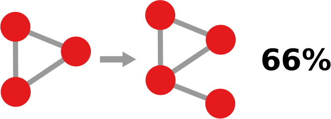
(on the left we have the “friend of my friend” situation, while on the right we have the “enemy of my enemy” rule). On the other hand, these structures are unbalanced:

(the latter on the right is actually a bit more complicated situation, but our dive in social balance is coming to an abrupt end, therefore we have no space to deal with it).

These structures are indeed found, as expected, to be over- or under-expressed in real world social networks (see the work of Szell et al). So the state of the art of link sign classification simply takes an edge, it controls for all the triangles surrounding it and returns the expected edge (here’s the paper – to be honest there are other papers with different proposed techniques, but this one is the most successful).

Now, the critique. This approach in my opinion has two major flaws. First, it is too deterministic. By applying social balance theory we are implying that all social networks obey to the very same mechanics even if they appear in different contexts. My intuition is that this assumption is rather limiting and untrue. Second, it limits itself to simple structures, i.e. triads of three nodes and edges. It does so because triangles are easy to understand for humans, because they are described by the very intuitive sentences presented before. But a computer does not need this oversimplification: a computer is there to do the work we find too tedious to do (remember the introduction: computer scientists are lazy animals).

In the last months, I worked on this problem with a very smart undergraduate student for his master thesis (this is the resulting paper, published this year at SocialCom). Our idea was (1) to use graph mining techniques to count not only triangles but any kind of structures in signed complex networks. Then, (2) we generated graph association rules using the frequencies of the structures extracted and (3) we used the rules with highest confidence and support to classify the edge sign. Allow me to decode in human terms what I just described technically.

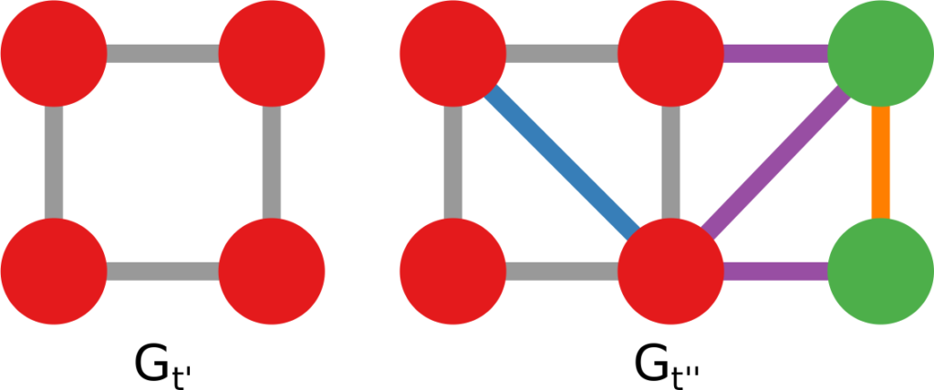
1) Graph mining algorithms are algorithms that, given a set of small graphs, count in how many of the graphs a particular substructure is present. The first problem is that these algorithms are not really well defined if we have a single graph for which we want to count how many times the structure is present*. Unfortunately, what we have is indeed not a collection of small graphs, but a single large graph, like this:

So, the first step is to split this structure in many small graphs. Our idea was to extract the ego network for each node in the network, i.e. the collection of all the neighbors of this node, and the edges among them. The logical explanation is that we count how many users “see” the given structure around them in the network:

(these are only 4 ego networks out of a total of 20 from the above example).

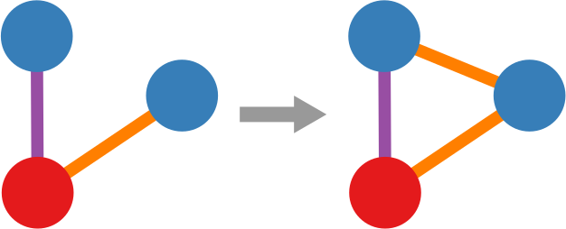
2) Now we can count how many times, for example, a triangle with three green edges is “seen” by the nodes of the network. Now we need to construct the “graph association rule”. Suppose that we “see” the following graph 20 times:

and the following graph, which is the same graph but with one additional negative edge, 16 times:

In this case we can create a rule stating: whenever we see the former graph, then we know with 80% confidence (16 / 20 = 0.8) that this graph is actually part of the latter one. The former graph is called premise and the latter is the consequence. We create rules in such a way that the consequence is an expansion of just one edge of the premise.

3) Whenever we want to know if we can trust the new guy (i.e. we have a mysterious edge without the sign), we can check around what premises match.  The consequences of these premises give us a hunch at the sign of our mysterious edge and the consequence with highest confidence is the one we will use to guess the sign.

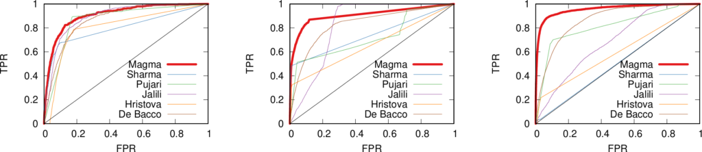
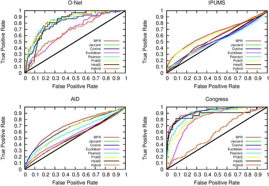
In the paper you can find the details of the performance of this approach. Long story short: we are not always better than the approach based on social balance theory (the “triangle theory”, as you will remember). We are better in general, but worse when there are already a lot of friends with an expressed opinion about the new guy**. However, this is something that I give away very happily, as usually they don’t know, because social networks are sparse and there is a high chance that the new person does not share any friends with you. So, here’s the catch. If you want to answer the initial question the first thing you have to do is to calculate how many friends of yours have an opinion. If few do (and that happens most of the time) you use our method, otherwise you just rely on them and you trust the social balance theory.

With our approach we overcome the problems of determinism and oversimplification I stated before, as we generate different sets of rules for different networks and we can generate rules with an arbitrary number of nodes. Well, we could, as for now this is only a proof of principle. We are working very hard to provide some usable code, so you can test yourself the long blabbering present in this post.


* Note for experts in graph mining: I know that there are algorithms defined on the single-graph setting, but I am explicitly choosing an alternative, more intuitive way.

** Another boring formal explanation. The results are provided in function of a measure called “embeddedness” of an edge (E(u,v) for the edge connecting nodes u and v). E(u,v) is a measure returning the number of common neighbors of the two nodes connected by the mysterious edge. For all the edges with minimum embeddedness larger than zero (E(u,v) > 0, i.e. all the edges in the network) we outperform the social balance, with accuracy close to 90%. However, for larger minimum embeddedness (like E(u,v) > 25), social balance wins. This happens because there is a lot of information around the edge. It is important to note that the number of edges with E(u,v) > 25 is usually way lower than half of the network (from 4% to 25%).

Continue Reading