Michele Coscia

If you follow this blog, you know that I periodically talk about community discovery. The problem seems so deceptively simple: finding groups of nodes densely connected in a network. If it is so simple, why have I been talking about it since 2012? The reason is that it isn’t so simple, and people have tried to organize the literature explaining how the thousands of different algorithms work, how they perform, what definition of “community” they use. After all that work, I’m still left with one question. Which two algorithms return the same gosh darned communities in a network? That’s what we’re going to discover today.

What I want to do is to take as many community discovery algorithms as I can, test them on a set of networks, and compare their results to estimate how similar they are. This gives me a similarity matrix of algorithms, which I can transform into a network by keeping only similarities that are statistically significant. Once I have the network, I can discovery groups of algorithms returning a coherent set of results, because they’re all significantly related to each other. How do I find these groups? Well, by ehm…. er… performing… community… discovery? on the… network of… community discovery… algorithms… This is exactly the outline of my paper Discovering Communities of Community Discovery, which I presented at ASONAM last month.

“As many community discovery algorithms as I can” turned out to be 73, all implemented in different languages, taking input in different ways, and providing different output formats. I ran them on more than 1,500 networks (real world ones from ICON and synthetic benchmarks). It was a… difficult month for me. I compared their partitions by estimating their mutual information: given that I know the results of algorithm A, how much can I infer about the results of algorithm B? For each network where two algorithms result in a lot of mutual information, I increase their similarity count by one. Once I have all similarity counts, I can extract the backbone of this matrix, controlling for the fact that some algorithms tend to be more peculiar than others, while others tend to be more mainstream.

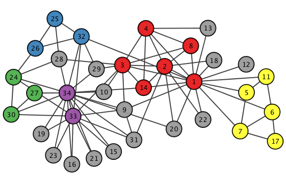
And this is the result (click to enlarge):

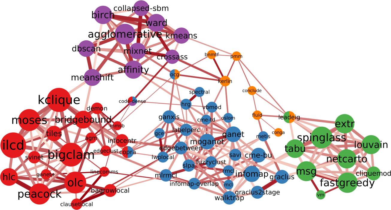
I love this network, because it has well defined groups and they all make sense. There’s the group of modularity maximization algorithms (in green), there’s the ones based on percolation / random walks (in blue), and the ones using neighbor similarity (in purple) as the guiding principle.

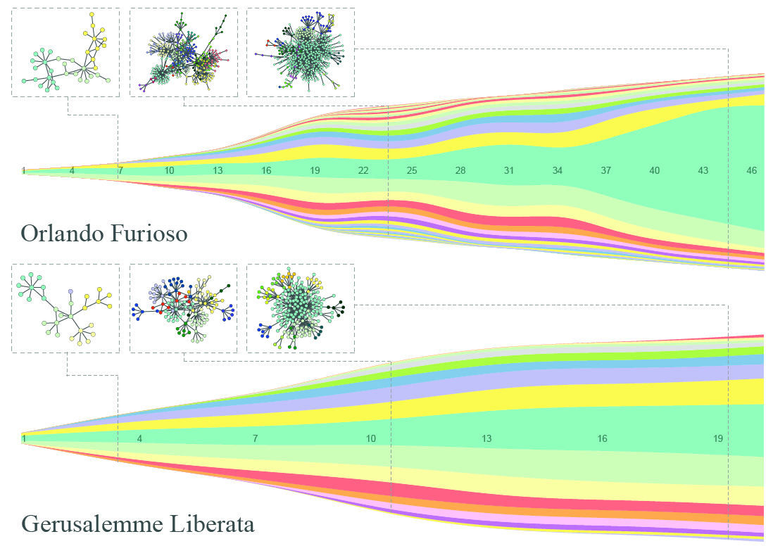
Then there’s a lump of algorithms that allow communities to share nodes (in red). The only thing these algorithms have in common is that they allow communities to share nodes, which is not a good enough common characteristics. The ways they find communities are as diverse as the ones you find in the rest of the network. But that’s the beauty of my approach: I can select a subset of nodes — say all overlapping community discovery algorithms — and re-apply the test of statistical significance with a more stringent threshold. This allows me to zoom in and see if there are meaningful structures inside the community. Lo and behold:

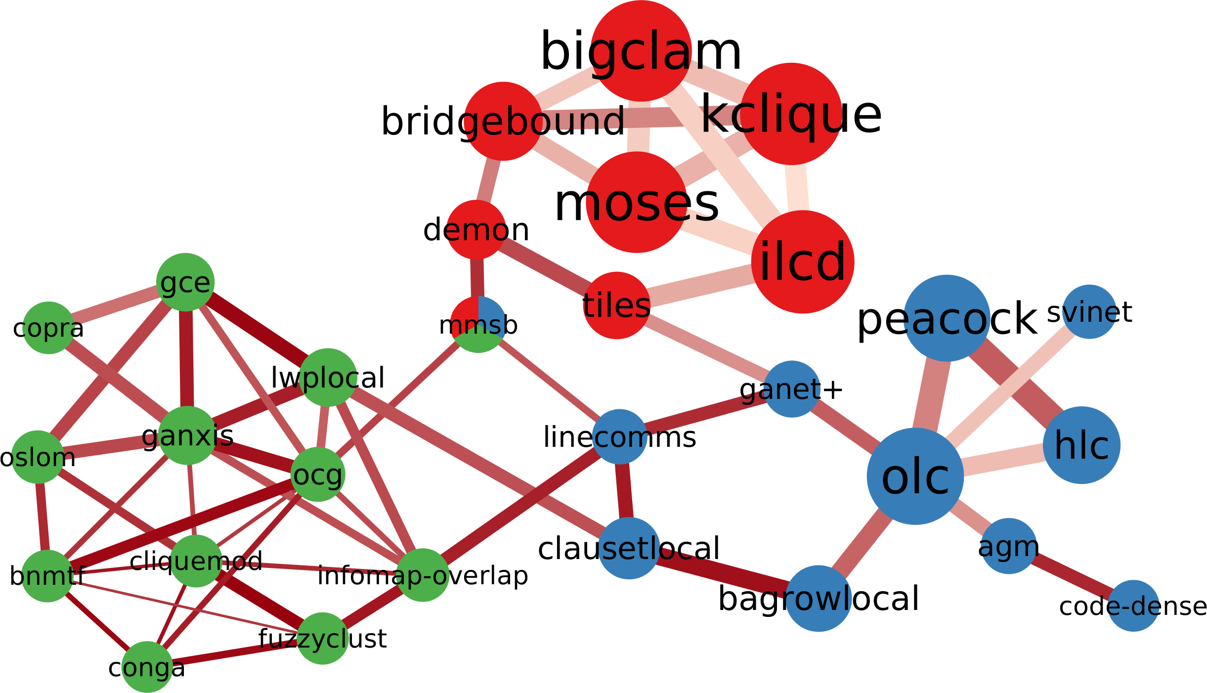
Here you can see meaningful groups of overlapping algorithms. There’s the ones achieving overlap by clustering edges instead of nodes (in blue), and the ones applying the percolation / random walk strategy (in green), but allowing for node sharing.

Why is this work significant? First, because it proves that there really are different — and valid — definitions of what communities are in complex networks. If there weren’t, this network would be more homogeneous, without distinct groups.

Second, as I mentioned, some of the networks I tested the algorithms on are standard benchmarks: LFR networks. These benchmarks grow a network with a planted community structure: the real latent structure the algorithm is supposed to find. Yet, this “ground truth” is well embedded in one of the clusters: the percolation/random walk community (in blue). LFR benchmarks follow that specific definition and not others. If you are developing a new community discovery algorithm which has a different community definition, you should not use the LFR benchmark to test it. Moreover, if you are developing a percolation/random walk algorithm and you’re correctly testing it on an LFR benchmark, you cannot test it against algorithms that are not part of the blue community. Otherwise the test would be unfair, because those algorithms are looking for something else: of course they’ll perform poorly on LFR benchmarks!

You can get the full list of algorithms that I tested, with proper references, from the official page of the project. From there, you can also download the network and use it for your purposes. This is necessarily an eternal work in progress: there are more than 73 community discovery algorithms out there. But I am but a man^{[citation needed]} and I cannot spend my entire time scouting for implementations on the web. I got to put bread (or, preferably, pasta) on the table as well. Thus, if you think I really should have included your algorithm in this structure, you can mail me and send me a working implementation of it, and I’ll gladly run it on my benchmarks.

What’s next? I’d be delighted to inaugurate the field of meta-research. So join me, as I develop new projects such as:

• Predicting links of link predictors: which link prediction algorithms will become more similar in the future?
• Spreading epidemics of epidemic spreading: which researchers will cave in to peer pressure and publish a paper studying the diffusion of some phenomenon?
• Modeling the growth of growth models: how has the Barabasi and Albert model evolved over time? Which features were added? What about Watts & Strogatz’s model?

(In case you were wondering, I’m joking. In network science, sometimes that might be hard to tell.)

(Or am I?)

(It’s settled: the best among these papers will receive the hereby instituted Escher prize, awarded by Douglas Hofstadter himself)

Continue Reading

I’m coming out of a long hiatus to write a quick post about a nice little paper I just put together with Riccardo Guidotti. The topic today is community discovery: the task of grouping nodes in a network because they connect to each other more strongly than with the other nodes in a network. No, wait, the actual topic is transactional data clustering: the task of grouping customers of a supermarket because they usually buy the same stuff. Wait what? What do these problems have to do with each other? Well, that’s what we concluded: the two things can be the same.

The title of the paper is “On the Equivalence between Community Discovery and Clustering” and it was accepted for publication at the GoodTechs conference in Pisa. The starting point of this journey was peculiar. Riccardo, being the smart cookie he is, published earlier this year a paper in the prestigious SIGKDD conference. In the paper, he and coauthors describe the Tx-means algorithm, that does exactly what I said before: it looks at the shopping carts of people, and figures out which ones are similar to each other. You can use it to give suggestions of items to buy and other nice applications. There is a three-minute video explaining the algorithm better than I can, which incidentally also shows that Riccardo has some serious acting chops, as a side of his research career:

The title of the paper is “Clustering Individual Transactional Data for Masses of Users” and you should check it out. So the question now is: how can I make all of this about me? Well, Riccardo wanted some help to break into the community discovery literature. So he asked my advice. My first advice was: don’t. Seriously, it’s a mess. He didn’t follow it. So the only option left was to help him out.

The main contribution of the paper is to propose one of the possible ways in which transactional data clustering can be interpreted as community discovery. The two tasks are known to be very similar in the literature, but there are many ways to map one onto the other, with no clear reason to prefer this or the other translation. In this paper, we show one of those translations, and some good reasons why it’s a good candidate. Now, the article itself looks like a five year old took a bunch of Greek letters from a bag and scattered them randomly on a piece of paper, so I’ll give you a better intuition for it.

The picture shows you transactional data. Each cart contains items. As the video points out, this type of data can also represent other things: a cart could be a user and the items could be the webpages she read. But we can go even more abstract than that. There is no reason why the items and the carts should be different entity types. A cart can contain… carts. We can define it as the list of carts it is related to, for any arbitrary relatedness criterion you’re free to choose (maybe it’s because they are cart-friends or something).

Once we do that, we can pivot our representation. Now it’s not transactional data any more: it is an edge list. Each node (the cart) lists the other nodes (cart-items) to which it connects. So this is a network — as shown below. What would it mean to find communities in this network? Well, it would mean — as I said at the beginning — to find groups of nodes that connect to each other. Or, in other words, group of carts that contain the same items (carts). Which is what Tx-means does.

This approach is a bit of a bastardization of community discovery because, if we apply it, then the community definition shifts from “densely connected nodes” to “similarly connected nodes.” But that’s a valid community definition — and that’s why community discovery is a mess — so we get a pass. It’s more or less the same thing I did on another working paper I’m sweating on, and so far only one person has called me out on that (thanks Adam), so I call it a success.

Why on Earth would we want to do this? Well, because Tx-means comes with some interesting advantages. First, let’s pitch it against some state of the art community discovery methods. In our experiments, Tx-means was the best at guessing the number of communities in networks of non-trivial size. This came without a big penalty in their Normalized Mutual Information — which measures how aligned the discovered communities are to the “real” communities as we gather them from metadata.

More importantly — as you saw in the video — Tx-means is able to extract “typical carts.” Translated into network lingo: with Tx-means you can extract the prototypical nodes of the community, or its most representative members. This has a number of applications if you are interested in, for instance, knowing who are the leaders, around which the nodes in the community coalesce. They are highlighted in colors in the picture above. You cannot really do this with Infomap, for instance.

So that’s the reason of this little exercise. Other transactional data clustering algorithms can use the same trick to go from carts to nodes, and therefore translate their features into the context of community discovery. Features that might be missing from the traditional algorithms we use to detect communities.

 

Continue Reading

You need to forgive me for the infamous click-bait title I gave to the post. You literally need to, because you have to save your hate for the actual topic of the post, which is Big Data. Or whatever you want to call the scenario in which scientists are flooded with so much data that traditional approaches break, for one reason or another. I like to use the Big Data label just because it saves time. One of the advantages of Big Data is that it’s useful. Once you can manage it, simple analysis will yield great profits. Take Google Translate: it does not need very sophisticated language models because millions of native speakers will contribute better translations, and simple Bayesian updates make it works nicely.

Of course there are pros and cons. I am personally very serious about the pros. I like Big Data. Exactly because of that love, honesty pushes me to find the limits and scrutinize the cons of Big Data. And that’s today’s topic: “yet another person telling you why Big Data is not such a great thing (even if it is, sometimes)” (another very good candidate for a click-bait title). The occasion for such a shameful post is the recent journal version of my work on human mobility borders (click for the blog post where I presented it). In that work we analysed the impact of geographic resolution on mobility data to locate the real borders of human mobility. In this updated version, we also throw temporal resolution in the mix. The new paper is “Spatial and Temporal Evaluation of Network-Based Analysis of Human Mobility“. So what does the prediction of human mobility have to do with my blabbering about Big Data?

Big Data is founded on the idea that more data will increase the quality of results. After all, why would you gather so much data at the point of not knowing how to manage them if it was not for the potential returns? However, sometimes adding data will actually decrease the research quality. Take again the Google Translate example: a non native speaker could add noise, providing incorrect translations. In this case the example does not really hold, because it’s likely that the vast majority of contributions comes from people who are native speakers in one of the two languages involved. But in my research question about human mobility it still holds. Remember what was the technique in the paper: we have geographical areas and we consider them nodes in a network. We connect nodes if people travel from an area to another.

Let’s start from a trivial observation. Weekends are different from weekdays. There’s sun, there’s leisure time, there are all those activities you dream about when you are stuck behind your desk Monday to Friday. We expect to find large differences in the networks of weekdays and in the networks of weekends. Above you see three examples (click for larger resolution). The number of nodes and edges tells us how many areas are active and connected: there are much fewer of them during weekends. The number of connected components tells us how many “islands” there are, areas that have no flow of people between them. During weekends, there are twice as much. The average path length tells us how many connected areas you have to hop through on average to get from any area to any other area in the network: higher during weekdays. So far, no surprises.

If you recall, our objective was to define the real borders of the macro areas. In practice, this is done by grouping together highly connected nodes and say that they form a macro area. This grouping has the practical scope of helping us predict within which border an area will be classified: it’s likely that it won’t change much from a day to another. The theory is that during weekends, for all the reasons listed before (sun’n’stuff), there will be many more trips outside of a person’s normal routine. By definition, these trips are harder to predict, therefore we expect to see lower prediction scores when using weekend data.

The first part of our theory is proven right: there are indeed much less routine trips during weekends. Above we show the % of routine trips over all trips per day. The consequences for border prediction hold true too. If you use the whole week data for predicting the borders of the next week you get poorer prediction scores. Poorer than using weekday data for predicting weekday borders. Weekend borders are in fact much more volatile, as you see below (the closer the dots to the upper right corner, the better the prediction, click for higher resolution):

In fact we see that the borders are much crazier during weekends and this has a heavy influence on the whole week borders (see maps below, click for enjoying its andywarholesque larger resolution). Weekends have a larger effect on our data (2/7), much more than our example in Google Translate.

The conclusion is therefore a word of caution about Big Data. More is not necessarily better: you still need theoretical grounds when you add data, to be sure that you are not introducing noise. Piling on more data, in my human mobility study, actually hides results: the high predictability of weekday movements. It also hides the potential interest of more focused studies about the mobility during different types of weekends or festivities. For example, our data involves the month of May, and May 1st is a special holiday in Italy. To re-ignite my Google Translate example: correct translations in some linguistic scenarios are incorrect otherwise. Think about slang. A naive Big Data algorithm could be caught in between a slang war, with each faction claiming a different correct translation. A smarter, theory-driven, algorithm will realize that there are slangs, so it will reduce its data intake to solve the two tasks separately. Much better, isn’t it?

Continue Reading

The literature about community discovery, which deals with the problem of finding related groups of nodes in a network, is vast, interesting and full of potential practical applications. However, if I would have to give one critique of it, it would be about its self referential character. Most community discovery papers I read in computer science and physics journals are mainly about finding communities. Not much time is spent thinking about what to do with them, or what they mean. My first post in this blog was about a community discovery algorithm. Recently, an extended version of that paper has been accepted in a computer science journal. Since that first post, I (mainly) added some crucial modifications and features to the algorithm. I don’t want to talk about those here: they are boring. I also didn’t bring up this paper to boast about it. Okay, maybe a little. I did it because the paper touches upon the issue I am talking about here: it tries to do something with communities, it tries to explain something about them. Namely, it asks: why do communities overlap?

First of all: communities do overlap. When trying to detect them, many researchers realized that hard partitions, where each node can belong to one and only one community, are not always a good idea. Most of them found this a problem. Others were actually very happy: the problem gets harder! Nice! (Researchers are weird). Blinded by their enthusiasm, they started developing algorithms to deal with this overlap. Not many asked the question I am trying to answer here: why do communities overlap? As a result, some of these algorithms detect this overlap, but using approaches that do not really mean anything in real life, it’s just a mathematical trick. Others, instead, build the algorithm around a core hypothesis.

This hypothesis is nothing unheard of. Communities overlap because people have complex lives. Some of your college mates also attend your yoga class. And you know your significant other’s colleagues, which puts you in their community. All these communities have you as common member, and probably some more people too. The beauty of this is that it is not only intuitive: it works well in finding communities in real world social networks. So well that it is the assumption of my approach and of many others outstanding algorithms (this and this are the first two that pop into my mind, but there are probably many more). Another beautiful thing about it is that it is almost obvious, and so it is probably true. But here we hit a wall.

The fact that it is simple, reasonable and it works well in practice proves nothing about its property of being true. There are things that are not simple nor reasonable, but nevertheless true (hello quantum physics!). And there is practical knowledge that does not quite correspond to how things work (in my opinion, most computer science is a patch and nobody really knows why it works). Unless we test it, we cannot say that this nice practical principle actually corresponds to something happening in reality. So how do we go on and prove it? In the paper I proposed a first step.

This brings me back to another old love of mine. Multidimensional networks. They are networks in which we put multiple relations in a cage together in mating season and see what happens (research is fun). The idea behind the paper is that multidimensional networks give us the perfect tool to test the hypothesis. In monodimensional networks you have no clue why two people are connecting besides the obvious “they know each other”. In a multidimensional network, you know why they know each other, it’s information embedded in the type of the relation. So, the hypothesis is that different types of relations are the cause of the community overlap, and with multidimensional networks we can look at how communities distribute over relations. First, let us take a look at what two overlapping communities look like in a multidimensional network.

We collected a multidimensional social network putting together relationships between users in Facebook, Twitter and Foursquare. We then used DEMON to extract overlapping communities from each dimension. We then took two communities with extensive overlap in the Facebook dimension (picture below).

We then looked at the very same set of nodes, but now in the Foursquare network. In the picture below, we kept the edges, and the node positioning, of the Facebook network to make the comparison easier, but keep in mind that the edges in the Foursquare dimension are different, and they are the ones that decide to what community the nodes belong.

Very interesting. The communities look a lot alike, although the shared (and non shared) nodes are slightly different. Now node 7369 is shared (it wasn’t in Facebook) while node 8062 isn’t (whereas it was before). Let’s put another nail on the coffin and see the communities these nodes belong in Twitter (same disclaimer applies):