Michele Coscia

The Michelangelo Principle — almost certainly apocryphal — states that:

If you want to transform a marble block into David, just chip away the stone that doesn’t look like David.

This seems to be a great idea to solve literally every problem in the world: if you want to fix evil, just remove from the world everything that is evil. But I don’t want to solve every problem in the world. I want to publish papers on network analysis. And so I apply it to network analysis. In this case, I use it to answer the question whether a directed network has a hierarchical structure or not. The result has been published in the paper “Using arborescences to estimate hierarchicalness in directed complex networks“, which appeared last month in PLoS One.

To determine whether a network is hierarchical is useful in a number of applications. Maybe you want to know how resilient your organization is to the removal of key elements in the team. Or you want to prove that a system you mapped does indeed have a head, instead of being a messy blob. Or you want to know whether it is wise to attempt a takedown on the structure. In all these scenarios, you really desire a number between 0 and 1 that tells you how hierarchical the network is. This is the aim of the paper.

Following the Michelangelo Principle, I decide to take the directed network and chip away from it everything that does not look like a perfect hierarchy. Whatever I’m left with is, by definition, a perfect hierarchy. If I’m left with a significant portion of the original network, then it was a pretty darn good hierarchy to begin with. If I’m left with nothing, well, then it wasn’t a hierarchy at all. Easy. Let’s translate this into an algorithm. To do so, we need to answer a couple of questions:

1. What’s a “perfect hierarchy”?
2. How do we do the chipping?
3. How do we quantify the amount we chipped?

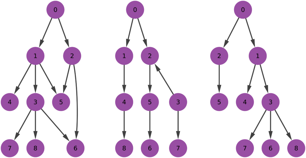
The first question is the one where we have most wiggle room. People might agree or disagree with the definition of perfect hierarchy that I came up with. Which is: a perfect hierarchy is a system where everybody answers to a single boss, except the boss of them all, who answers to no one. I like this definition because it solves a few problems.

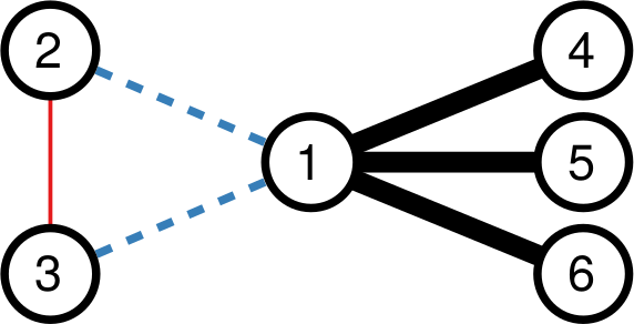
Consider the picture above. In the leftmost example, if we assume nodes 1 and 2 give contradictory orders, node 5 doesn’t really know what to do, and the idea of a hierarchy breaks down. In the example in the middle, we don’t even know who’s the boss of them all: is it node 0 or node 3? The rightmost example leaves us no doubt about who’s boss, and there’s no tension. For those curious, network scientists call that particular topology an “arborescence“, and that’s the reason this exotic word is in the paper title. Since this is a well defined concept, we know exactly what to remove from an arbitrary directed network to make it into an arborescence.

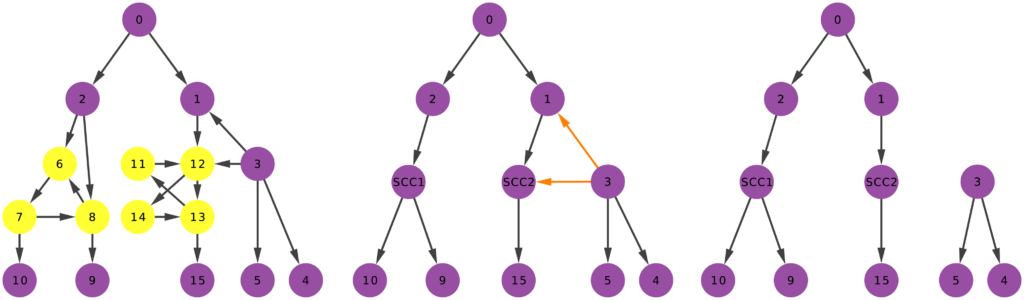
Time to chip! Arbitrary directed networks contain strongly connected components: they have paths that can lead you back to your origin if you follow the edge directions. An arborescence is a directed acyclic graph, meaning that it cannot have such components. So our first step is to collapse them (highlighted in yellow above) into a single node. Think of strongly connected components as headless teams where all the collaborators are at the same level. They are a node in the hierarchy. We don’t care how a node organizes itself internally. As long as it answers to a boss and gives direction to its underlings, it can do it in whichever way it wants.

Second chipping step: in an arborescence, all nodes have at most one incoming connection, and only one node has zero. So we need to remove all offending remaining edges (highlighted in orange above). Once we complete both steps, we end up with an arborescence, and we’re done. (There are edge cases in which you’ll end up with multiple weakly connected components. That’s fine. If you follow the procedure, each of these components is an arborescence. Technically speaking, this is an “arborescence forest”, and it is an acceptable output)

We can now answer the final question: quantifying how much we chipped. I decide to focus on the number of edges removed. Above, you see that the original graph (left) had twenty edges, and that (right) nine edges survived. So the “hierarchicalness” of the original graph is 9 / 20 = .45.

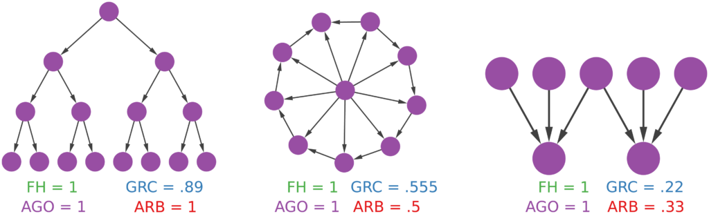
Now the question is: why would someone use this method to estimate a network’s degree of hierarchicalness and not one of the many already proposed in the literature? The other methods all have small downsides. I build some toy examples where I can show that arborescence is the way to go. For instance, you can’t find a more perfect hierarchy than a balanced tree (leftmost example above). However, Global Reach Centrality would fail to give it a perfect score — since it thinks only a star graph is a perfect hierarchy. Agony and Flow Hierarchy aren’t fooled in this case, but give perfect scores in many other scenarios: a wheel graph with a single flipped edge (example in the middle), or a case where there are more bosses than underlings (rightmost example). Those who have been in a team with more bosses than workers know that the arrangement could be described in many ways, but “perfect” ain’t one of them.

Arborescence is also able to better distinguish between purely random graphs and graphs with a hierarchy — such as a preferential attachment with edges going from the older to the newer nodes (details in the paper). Before you start despairing, it’s not that I’m saying we’ve been doing hierarchy detection wrong for all these years. In most real world scenarios, these measures agree. But, when they disagree, arborescence is the one that most often sides with the domain experts, who have well informed opinions whether the system represented by the network should be a hierarchy or not.

To conclude, this method has several advantages over the competitors. It’s intuitive: it doesn’t give perfect ratings to imperfect hierarchies and vice versa. It’s graphic: you can easily picture what’s going on in it, as I did in this blog post. It’s conservative: it doesn’t make the outlandish claim that “everyone before me was a fool”. It’s rich: it gives you not only a score, but also a picture of the hierarchy itself. So… Give it a try! The code is freely available, and it plays nicely with networkx.

Continue Reading

Networks are a fantastic tool for understanding an interconnected world. But, to paraphrase Spider Man, with networks’ expressive power come great headaches. Networks lure us in with their promise of clearly representing complex phenomena. However, once you start working with them, all you get is a tangled mess. This is because, most of the time, there’s noise in the data and/or there are too many connections: you need to weed out the spurious ones. The process of shaving the hairball by keeping only the significant connections — the red ones in the picture below —  is called “network backboning”. The network backbone represents the true relationships better and will play much nicer with other network algorithms. In this post, I describe a backboning method I developed with Frank Neffke, from the paper “Network Backboning with Noisy Data” accepted for publication in the International Conference on Data Engineering (the code implementing the most important backbone algorithms is available here).

Network backboning is as old as network analysis. The first solution to the problem was to keep edges according to their weight. If you want to connect people who read the same books, pairs who have few books in common are out. Serrano et al. pointed out that edge weight distributions can span many orders of magnitude — as shown in the figure below (left). Even with a small threshold, we are throwing away a lot of edges. This might not seem like a big deal — after all we’re in the business of making the network sparser — except that the weights are not distributed randomly. The weight of an edge is correlated with the weights of the edges sharing a node with it — as shown by the figure below (right). It is easy to see why: if you have a person who read only one book, all its edges can have at most weight one.

Their weights might be low in comparison with the rest of the network, but they are high for their nodes, given their propensity to connect weakly. Isolating too many nodes because we accidentally removed all their edges is a no-no, so Serrano and coauthors developed the Disparity Filter (DF): a technique to estimate the significance of one node’s connections given its typical edge weight, regardless of what the rest of the network says.

This sounds great, but DF and other network backboning approaches make imprecise assumptions about the possibility of noise in our estimate of edge weights. In our book example, noise means that a user might have accidentally said that she read a book she didn’t, maybe because the titles were very similar. One thing DF gets wrong is that, when two nodes are not connected in the raw network data, it would say that measurement error is absent. This is likely incorrect, and it screams for a more accurate estimate of noise. I’m going to leave the gory math details in the paper, but the bottom line is that we used Bayes’ rule. The law allows us to answer the question: how surprising is the weight of this edge, given the weights of the two connected nodes? How much does it defy my expectation?

The expectation here can be thought of as an extraction without replacement, much like Bingo (which statisticians — notorious for being terrible at naming things — would call a “hypergeometric” one). Each reader gets to extract a given number of balls (n, the total number of books she read), drawing from a bin in which all balls are the other users. If a user read ten books, then there are ten balls representing her in the bin. This is a good way to have an expectation for zero edge weights (nodes that are not connected), because we can estimate the probability of never extracting a ball with a particular label.

I highlighted the words one and two, because they’re a helpful key to understand the practical difference between the approaches. Consider the toy example below. In it, each edge’s thickness is proportional to its weight. Both DF and our Noise Corrected backbone (NC) select the black edges: they’re thick and important. But they have different opinions about the blue and red edges. DF sees that nodes 2 and 3 have mostly weak connections, meaning their thick connection to node 1 stands out. So, DF keeps the blue edges and it drops the red edge. It only ever looks at one node at a time.

NC takes a different stance. It selects the red edge and drops the blue ones. Why? Because for NC what matters more is the collaboration between the two nodes. Sure, the blue connection is thicker than the red one. But node 1 always has strong connections, and its blue edges are actually particularly weak. On the other hand, node 3 usually has weak connections. Proportionally speaking, the red edge is more important for it, and so it gets saved.

To sum up, NC:

1. Refines our estimate of noise in the edge weights;
2. Sees an edge as the collaboration between two nodes rather that an event happening to one of them;
3. Uses a different model exploiting Bayes’ law to bake these aspects together.

How does that work for us in practice? Above you see some simulations made with artificial networks, of which we know the actual underlying structure, plus some random noise — edges thrown in that shouldn’t exist. The more noise we add the more difficult it is to recover the original structure. When there is little noise, DF (in blue) is better. NC (in red) starts to shine as we increase the amount of noise, because that’s the scenario we were targeting.

In the paper we also show that NC backbones have a comparable stability with DF, meaning that extracting the backbone from different time snapshots of the same phenomenon usually does not yield wildly different results. Coverage — the number of nodes that still have at least one edge in the network — is also comparable. Then we look at quality. When we want to predict some future relationship among the nodes, we expect noisy edges to introduce errors in the estimates. Since a backbone aims at throwing them away, it should increase our predictive power. The table below (click it to enlarge) shows that, in different country-country networks, the predictive quality (R²) using an NC backbone is higher than the one we get using the full noisy network. The quality of prediction can get as high as twice the baseline (the table reports the quality ratio: R² of the backbone over R² of the full network, for different methods).

The conclusion is that, when you are confident about the measurement of your network, you should probably extract its backbone using DF. However, in cases of uncertainty, NC is the better option. You can test it yourself!

Continue Reading

Complex networks can come in different flavors. As you know if you follow this blog, my signature dish is multilayer/multidimensional networks: networks with multiple edge types. One of the most popular types is bipartite networks. In bipartite networks, you have two types of nodes. For example, you can connect users of Netflix to the movies they like. As you can see from this example, in bipartite networks we allow only edges going from one type of nodes to the other. Users connect to movies, but not to other users, and movies can’t like other movies (movies are notoriously mean to each other).

Many things (arguably almost everything) can be represented as a bipartite network. An occupation can be connected to the skills and/or tasks it requires, an aid organization can be connected to the countries and/or the topics into which it is interested, a politician is connected to the bills she sponsored. Any object has attributes. And so it can be represented as an object-attribute bipartite network. However, most of the times you just want to know how similar two nodes of the same type are. For example, given a movie you like, you want to know a similar movie you might like too. This is called link prediction and there are two ways to do this. You could focus on predicting a new user-movie connection, or focus instead on projecting the bipartite network to discover the previously unknown movie-movie connections. The latter is the path I chose, and the result is called “Network Map”.

It is clearly the wrong choice, as the real money lies in tackling the former challenge. But if I wanted to get rich I wouldn’t have chosen a life in academia anyway. The network map, in fact, has several advantages over just predicting the bipartite connections. By creating a network map you can have a systemic view of the similarities between entities. The Product Space, the Diseasome, my work on international aid. These are all examples of network maps, where we go from a bipartite network to a unipartite network that is much easier to understand for humans and to analyze for computers.

Creating a network map, meaning going from a user-movie bipartite network to a movie-movie unipartite network, is conceptually easy. After all, we are basically dealing with objects with attributes. You just calculate a similarity between these attributes and you are done. There are many similarities you can use: Jaccard, Pearson, Cosine, Euclidean distances… the possibilities are endless. So, are we good? Not quite. In a paper that was recently accepted in PLoS One, Muhammed Yildirim and I showed that real world networks have properties that make the general application of any of these measures quite troublesome.

For example, bipartite networks have power-law degree distributions. That means that a handful of attributes are very popular. It also means that most objects have very few attributes. You put the two together and, with almost 100% probability, the many objects with few attributes will have the most popular attributes. This causes a great deal of problems. Most statistical techniques aren’t ready for this scenario. Thus they tend to clutter the network map, because they think that everything is similar to everything else. The resulting network maps are quite useless, made of poorly connected dense areas and lacking properties of real world networks, such as power-law degree distributions and short average path length, as shown in these plots:

Of course sometimes some measure gets it right. But if you look closely at the pictures above, the only method that consistently give the shortest paths (above, when the peak is on the left we are good) and the broadest degree distributions (below, the rightmost line at the end in the lower-right part of the plot is the best one) is the red line of “BPR”. BPR stands for “Bipartite Projection via Random-walks” and it happens to be the methodology that Muhammed and I invented. BPR is cool not only because its network maps are pretty. It is also achieving higher scores when using the network maps to predict the similarity between objects using ground truth, meaning that it gives the results we expect when we actually already know the answers, that are made artificially invisible to test the methodology. Here we have the ROC plots, where the highest line is the winner:

So what makes BPR so special? It all comes down to the way you discount the popular attributes. BPR does it in a “network intelligent” way. We unleash countless random walkers on the bipartite network. A random walker is just a process that starts from a random object of the network and then it jumps from it to one of its attributes. The target attribute is chosen at random. And then the walker jumps back to an object possessing that attribute, again choosing it at random. And then we go on. At some point, we start from scratch with a new random walk. We note down how many times two objects end up in the same random walk and that’s our similarity measure. Why does it work? Because when the walker jumps back from a very popular attribute, it could essentially go to any object of the network. This simple fact makes the contribution of the very popular attributes quite low.

BPR is just the latest proof that random walks are one of the most powerful tools in network analysis. They solve node ranking, community discovery, link prediction and now also network mapping. Sometimes I think that all of network science is founded on just one algorithm, and that’s random walks. As a final note, I point out that you can create your own network maps using BPR. I put the code online (the page still bears the old algorithm’s name, YCN). That’s because I am a generous coder.

Continue Reading

Imagine being subscribed to a service where you can read other users’ opinions about what interests you. Imagine that, for your convenience, the system allows you to tag other users as “reliable” or “unreliable”, such that the system will not bother you by signaling new opinions from users that you regard as unreliable, while highlighting the reliable ones. Imagine noticing a series of opinions, by a user you haven’t classified yet, regarding stuff you really care about. Imagine also being extremely lazy and unwilling to make up your own mind if her opinions are really worth your time or not. How is it possible to classify the user as reliable or unreliable for you without reading?

What I just described in the previous paragraph is a problem affecting only very lazy people. Computer Science is the science developed for lazy people, so you can bet that this problem definition has been tackled extensively. In fact, it has been. This problem is known as “Edge Sign Classification”, the art of classifying positive/negative relations in social media.

Computer Science is not only a science for lazy people, is also a science carried out by lazy people. For this reason, the edge sign classification problem has been mainly tackled by borrowing the social balance theory for complex networks, an approach that here I’m criticizing (while providing an alternative, I’m not a monster!). Let’s dive for a second into social balance theory, with the warning that we will stay on the surface without oxygen tanks, to get to the minimum depth that is sufficient for our purposes.

Formally, social balance theory states that in social environments there exist structures that are balanced and structures that are unbalanced. The former should be over-expressed (i.e. we are more likely to find them) while the latter should be rarer than expected. If these sentences are unclear to you, allow me to reformulate them using ancient popular wisdom. Social balance theory states mainly two sentences: “The friend of my friend is usually my friend too” and “The enemy of my enemy is usually my friend”, so social relations following these rules are more common than ones that do not follow them.

Let’s make two visual examples among the many possible. These structures in a social network are balanced:

(on the left we have the “friend of my friend” situation, while on the right we have the “enemy of my enemy” rule). On the other hand, these structures are unbalanced:

(the latter on the right is actually a bit more complicated situation, but our dive in social balance is coming to an abrupt end, therefore we have no space to deal with it).

These structures are indeed found, as expected, to be over- or under-expressed in real world social networks (see the work of Szell et al). So the state of the art of link sign classification simply takes an edge, it controls for all the triangles surrounding it and returns the expected edge (here’s the paper – to be honest there are other papers with different proposed techniques, but this one is the most successful).

Now, the critique. This approach in my opinion has two major flaws. First, it is too deterministic. By applying social balance theory we are implying that all social networks obey to the very same mechanics even if they appear in different contexts. My intuition is that this assumption is rather limiting and untrue. Second, it limits itself to simple structures, i.e. triads of three nodes and edges. It does so because triangles are easy to understand for humans, because they are described by the very intuitive sentences presented before. But a computer does not need this oversimplification: a computer is there to do the work we find too tedious to do (remember the introduction: computer scientists are lazy animals).

In the last months, I worked on this problem with a very smart undergraduate student for his master thesis (this is the resulting paper, published this year at SocialCom). Our idea was (1) to use graph mining techniques to count not only triangles but any kind of structures in signed complex networks. Then, (2) we generated graph association rules using the frequencies of the structures extracted and (3) we used the rules with highest confidence and support to classify the edge sign. Allow me to decode in human terms what I just described technically.

1) Graph mining algorithms are algorithms that, given a set of small graphs, count in how many of the graphs a particular substructure is present. The first problem is that these algorithms are not really well defined if we have a single graph for which we want to count how many times the structure is present*. Unfortunately, what we have is indeed not a collection of small graphs, but a single large graph, like this:

So, the first step is to split this structure in many small graphs. Our idea was to extract the ego network for each node in the network, i.e. the collection of all the neighbors of this node, and the edges among them. The logical explanation is that we count how many users “see” the given structure around them in the network:

(these are only 4 ego networks out of a total of 20 from the above example).

2) Now we can count how many times, for example, a triangle with three green edges is “seen” by the nodes of the network. Now we need to construct the “graph association rule”. Suppose that we “see” the following graph 20 times:

and the following graph, which is the same graph but with one additional negative edge, 16 times:

In this case we can create a rule stating: whenever we see the former graph, then we know with 80% confidence (16 / 20 = 0.8) that this graph is actually part of the latter one. The former graph is called premise and the latter is the consequence. We create rules in such a way that the consequence is an expansion of just one edge of the premise.

3) Whenever we want to know if we can trust the new guy (i.e. we have a mysterious edge without the sign), we can check around what premises match.  The consequences of these premises give us a hunch at the sign of our mysterious edge and the consequence with highest confidence is the one we will use to guess the sign.

In the paper you can find the details of the performance of this approach. Long story short: we are not always better than the approach based on social balance theory (the “triangle theory”, as you will remember). We are better in general, but worse when there are already a lot of friends with an expressed opinion about the new guy**. However, this is something that I give away very happily, as usually they don’t know, because social networks are sparse and there is a high chance that the new person does not share any friends with you. So, here’s the catch. If you want to answer the initial question the first thing you have to do is to calculate how many friends of yours have an opinion. If few do (and that happens most of the time) you use our method, otherwise you just rely on them and you trust the social balance theory.

With our approach we overcome the problems of determinism and oversimplification I stated before, as we generate different sets of rules for different networks and we can generate rules with an arbitrary number of nodes. Well, we could, as for now this is only a proof of principle. We are working very hard to provide some usable code, so you can test yourself the long blabbering present in this post.

* Note for experts in graph mining: I know that there are algorithms defined on the single-graph setting, but I am explicitly choosing an alternative, more intuitive way.

** Another boring formal explanation. The results are provided in function of a measure called “embeddedness” of an edge (E(u,v) for the edge connecting nodes u and v). E(u,v) is a measure returning the number of common neighbors of the two nodes connected by the mysterious edge. For all the edges with minimum embeddedness larger than zero (E(u,v) > 0, i.e. all the edges in the network) we outperform the social balance, with accuracy close to 90%. However, for larger minimum embeddedness (like E(u,v) > 25), social balance wins. This happens because there is a lot of information around the edge. It is important to note that the number of edges with E(u,v) > 25 is usually way lower than half of the network (from 4% to 25%).

Continue Reading