Michele Coscia

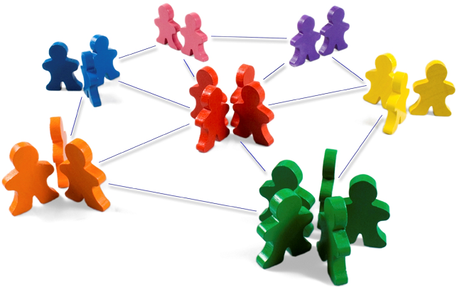
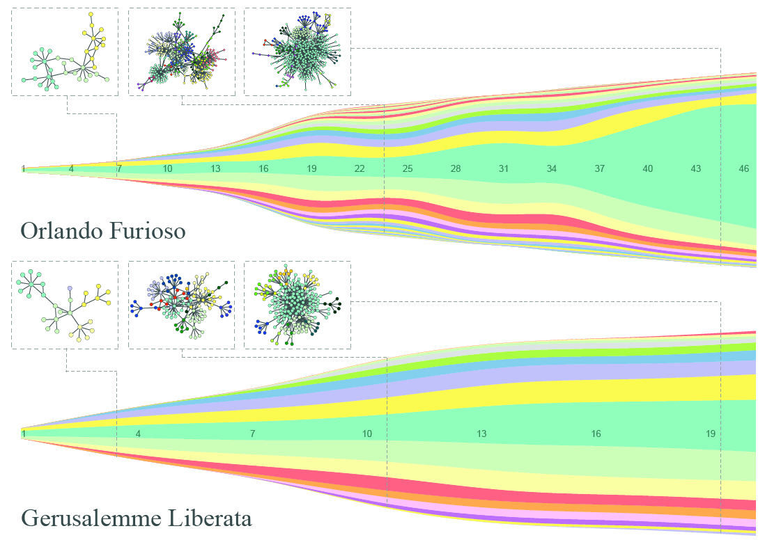
Complex networks can come in different flavors. As you know if you follow this blog, my signature dish is multilayer/multidimensional networks: networks with multiple edge types. One of the most popular types is bipartite networks. In bipartite networks, you have two types of nodes. For example, you can connect users of Netflix to the movies they like. As you can see from this example, in bipartite networks we allow only edges going from one type of nodes to the other. Users connect to movies, but not to other users, and movies can’t like other movies (movies are notoriously mean to each other).

Many things (arguably almost everything) can be represented as a bipartite network. An occupation can be connected to the skills and/or tasks it requires, an aid organization can be connected to the countries and/or the topics into which it is interested, a politician is connected to the bills she sponsored. Any object has attributes. And so it can be represented as an object-attribute bipartite network. However, most of the times you just want to know how similar two nodes of the same type are. For example, given a movie you like, you want to know a similar movie you might like too. This is called link prediction and there are two ways to do this. You could focus on predicting a new user-movie connection, or focus instead on projecting the bipartite network to discover the previously unknown movie-movie connections. The latter is the path I chose, and the result is called “Network Map”.

It is clearly the wrong choice, as the real money lies in tackling the former challenge. But if I wanted to get rich I wouldn’t have chosen a life in academia anyway. The network map, in fact, has several advantages over just predicting the bipartite connections. By creating a network map you can have a systemic view of the similarities between entities. The Product Space, the Diseasome, my work on international aid. These are all examples of network maps, where we go from a bipartite network to a unipartite network that is much easier to understand for humans and to analyze for computers.

Creating a network map, meaning going from a user-movie bipartite network to a movie-movie unipartite network, is conceptually easy. After all, we are basically dealing with objects with attributes. You just calculate a similarity between these attributes and you are done. There are many similarities you can use: Jaccard, Pearson, Cosine, Euclidean distances… the possibilities are endless. So, are we good? Not quite. In a paper that was recently accepted in PLoS One, Muhammed Yildirim and I showed that real world networks have properties that make the general application of any of these measures quite troublesome.

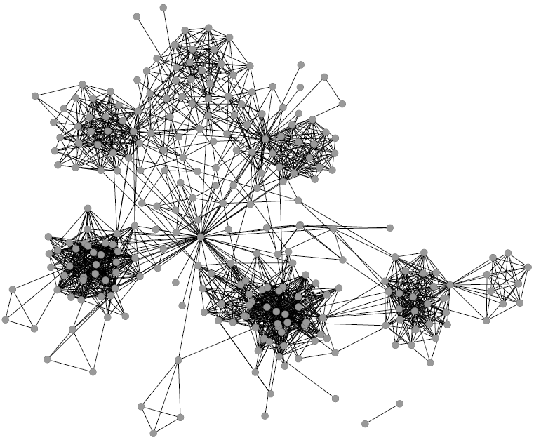
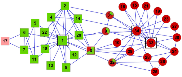
For example, bipartite networks have power-law degree distributions. That means that a handful of attributes are very popular. It also means that most objects have very few attributes. You put the two together and, with almost 100% probability, the many objects with few attributes will have the most popular attributes. This causes a great deal of problems. Most statistical techniques aren’t ready for this scenario. Thus they tend to clutter the network map, because they think that everything is similar to everything else. The resulting network maps are quite useless, made of poorly connected dense areas and lacking properties of real world networks, such as power-law degree distributions and short average path length, as shown in these plots:

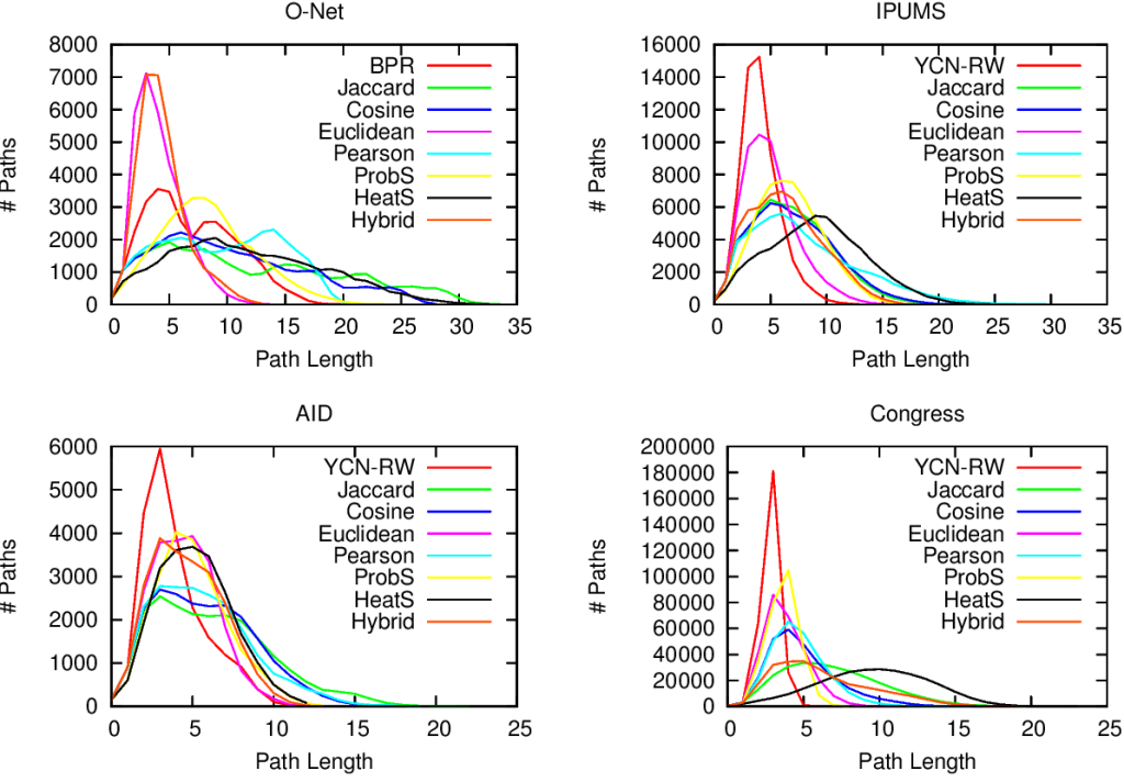
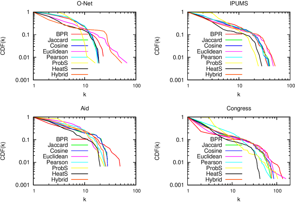
Of course sometimes some measure gets it right. But if you look closely at the pictures above, the only method that consistently give the shortest paths (above, when the peak is on the left we are good) and the broadest degree distributions (below, the rightmost line at the end in the lower-right part of the plot is the best one) is the red line of “BPR”. BPR stands for “Bipartite Projection via Random-walks” and it happens to be the methodology that Muhammed and I invented. BPR is cool not only because its network maps are pretty. It is also achieving higher scores when using the network maps to predict the similarity between objects using ground truth, meaning that it gives the results we expect when we actually already know the answers, that are made artificially invisible to test the methodology. Here we have the ROC plots, where the highest line is the winner:

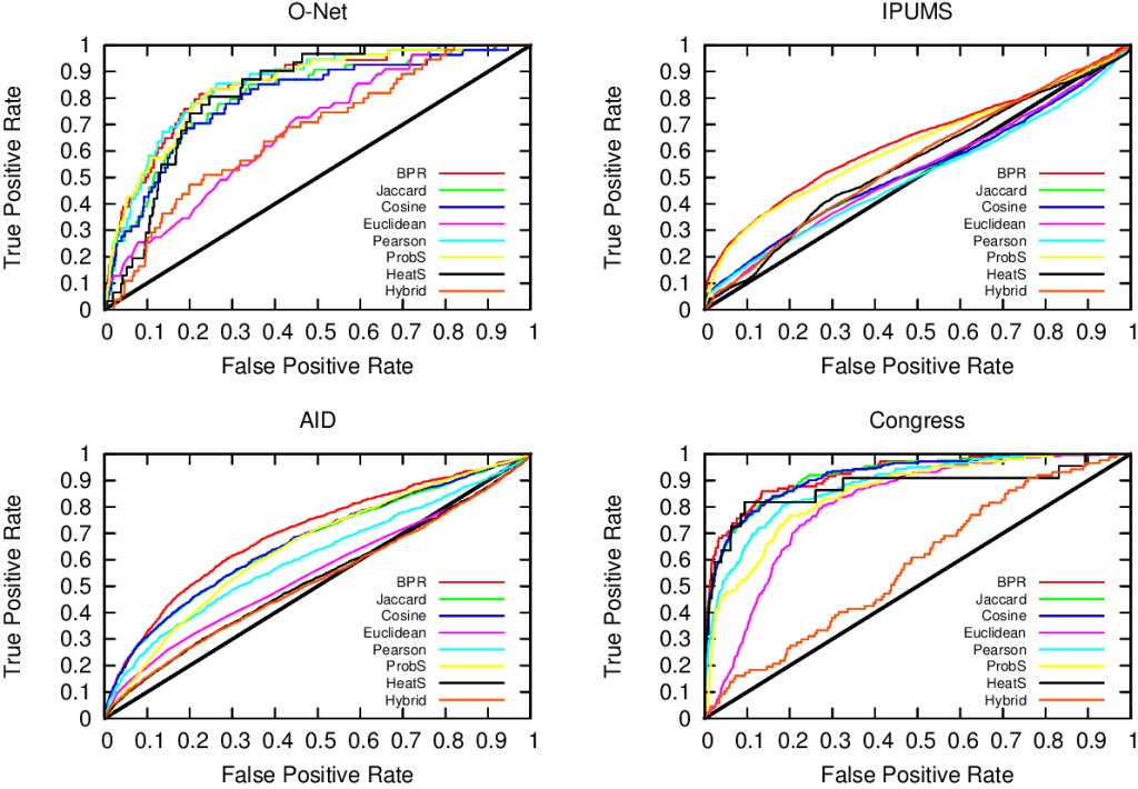
So what makes BPR so special? It all comes down to the way you discount the popular attributes. BPR does it in a “network intelligent” way. We unleash countless random walkers on the bipartite network. A random walker is just a process that starts from a random object of the network and then it jumps from it to one of its attributes. The target attribute is chosen at random. And then the walker jumps back to an object possessing that attribute, again choosing it at random. And then we go on. At some point, we start from scratch with a new random walk. We note down how many times two objects end up in the same random walk and that’s our similarity measure. Why does it work? Because when the walker jumps back from a very popular attribute, it could essentially go to any object of the network. This simple fact makes the contribution of the very popular attributes quite low.

BPR is just the latest proof that random walks are one of the most powerful tools in network analysis. They solve node ranking, community discovery, link prediction and now also network mapping. Sometimes I think that all of network science is founded on just one algorithm, and that’s random walks. As a final note, I point out that you can create your own network maps using BPR. I put the code online (the page still bears the old algorithm’s name, YCN). That’s because I am a generous coder.

For this end of July, I want to report some juicy facts about a work currently under development. Why? Because I think that these facts are interesting. And they are a bit depressing too. So instead of crying I make fun of them, because as the “Panic! At the Disco” would put it: I write sins, not tragedies.

So, a bit of background. Last year I got involved in an NSF project, with my boss Ricardo Hausmann and my good friend/colleague Prof. Stephen Kosack. Our aim is to understand what governments do. One could just pull out some fact-sheets and budgets, but in our opinion those data sources do not tell the whole story. Governments are complex systems and as complex systems we need to understand their emergent properties as collection of interacting parts. Long story short, we decided to collect data by crawling the websites of all public agencies for each US state government. As for why, you’ll have to wait until we publish something: the aim of this post is not to convince you that this is a good idea. It probably isn’t, at least in some sense.

It isn’t a good idea not because that data does not make sense. Au contraire, we already see it is very interesting. No, it is a tragic idea because crawling the Web is hard, and it requires some effort to do it properly. Which wouldn’t be necessarily a problem if there wasn’t an additional hurdle. We are not just crawling the Web. We are crawling government websites. (This is when in a bad horror movie you would hear a thunder nearby).

To make you understand the horror of this proposition is exactly the aim of this post. First, how many government websites are really out there? How to collect them? Of course I was not expecting a single directory for all US states. And I was wrong! Look for yourselves this beauty: http://www.statelocalgov.net/. The “About” page is pure poetry:

State and Local Government on the Net is the onle (sic) frequently updated directory of links to government sponsored and controlled resources on the Internet.

So up-to-date that their footer gets only to 2010 and their news section only includes items from 2004. It also points to:

SLGN Notes, a weblog, [that] was added to the site in June 2004. Here, SLGN’s editors comment on new, redesigned or updated state and local government websites, pointing out interesting or fun features for professional and consumer audiences alike and occasionally cover related news.

Yeah, go ahead and click the link, that is not the only 404 page you’ll see here.

Enough compliments to these guys! Let’s go back to work. I went straight to the 50 different state government’s websites and found in all of them an agency directory. Of course asking that these directories shared the same structure and design is too much. “What are we? Organizations whose aim is to make citizen’s life easier or governments?”. In any case from them I was able to collect the flabbergasting amount of 61,584 URLs. Note that this is six times as much as from statelocalgov.net, and it took me a week. Maybe I should start my own company 🙂

Awesome! So it works! Not so fast. Here we hit the first real wall of government technological incompetence. Out of those 61,584, only 50,999 actually responded to my pings. Please note that I already corrected all the redirects: if the link was outdated but the agency redirected you to the new URL, then that connection is one of the 50,999. Allow me to rephrase it in poetry: in the state government directories there are more than ten thousand links that are pure, utter, hopeless garbage nonsense. More than one out of six links in those directories will land you exactly nowhere.

Oh, but let’s stay positive! Let’s take a look at the ones that actually lead you somewhere:

• Inconsistent spaghetti-like design? Check. Honorable mention for the good ol’ frameset webdesign of http://colecounty.org/.
• Making your website an image and use <area> tag for links? Check. That’s some solid ’95 school.
• Links to websites left to their own devices and purchased by someone else? Check. Passing it through Google Translate, it provides pearls of wisdom like: “To say a word and wipe, There are various wipe up for the wax over it because wipe from”. Maybe I can get a half dozen of haiku from that page. (I have more, if you want it)
• ??? Check. That’s a Massachusetts town I do not want to visit.
• Maintenance works due to finish some 500 days ago? Check.
• Websites mysteriously redirected somewhere else? Check. The link should go to http://www.cityoflaplata.com/, but alas it does not. I’m not even sure what the heck these guys are selling.
• These aren’t the droids you’re looking for? Check.
• The good old “I forgot to renew the domain contract”? Check.

Bear in mind that this stuff is part of the 50,999 “good” URLs (these are scare quotes at their finest). At some point I even gave up noting down this stuff. I saw hacked webpages that had been there since years. I saw an agency providing a useful Google Maps of their location, which according to them was the middle of the North Pole. But all those things will be lost in time, like tears in the rain.

NetSci, the top global conference about network science, never fails to be a tornado of ideas. Now that the dust has settled, I feel a bit easier to put this year’s thoughts on this post. Yes, this is yet another conference report by yours truly.

Let’s first get over the mandatory part of the report: an evaluation of the awesomeness of the Multiple Networks satellite I co-organized with my friends scattered around Europe. As said, this year’s edition was open to submissions and we received 17 of them. I think that, as a start, that is a good figure. Also, the attendance was more than satisfactory, and it appears scattered only because we got the largest room of the conference! Here’s proof!

The overall event was a great success. The talks were very interesting and we had a great unexpected bonus point. One of our keynotes, as you might remember, was Mason Porter. Well, the guy actually got the Erdos-Renyi prize this year! The Erdos-Renyi prize has been established in 2012 and it goes to outstanding young researchers in network science. Well, make a note of this: speaking at the Multiple Networks satellite will eventually get you some important awards. After all, everybody knows that correlation = causation.

My favorite satellite (besides the one I organized, obviously) continues to be the Arts, Humanities and Complex Networks symposium. This year it was a little bit tougher than usual, with a lot of qualitative stuff that not everybody can appreciate. However, their keynote by Lada Adamic was nothing short of outstanding. She is currently working at Facebook, a position that gives her a privileged vantage point over memes and viral events. You know that those things tickle my curiosity very strongly, and Lada’s work is really great. She presented her work, where she proves that meme evolution and mutation on Facebook follows very closely the same mechanics of evolution and mutation we find in the biological world. Good news for my old paper, which was heading in the same direction!

Which brings me to the main conference, because one of the best talks I attended was from Jon Kleinberg, who collaborated with Lada on another memes-meet-Facebook work. In that case, there is less good news for me. My research plan is to use meme content to predict virality. However, the Kleinberg-Adamic dream team showed that content is actually a very weak factor! (Here’s a blog post about it).

There is still hope, though. My way to deal with content is fundamentally different than theirs. Plus the problem they are studying is slightly different from mine: they are analyzing memes that are already going viral and they want to know how popular they will get. I’m more focused on knowing if the meme is going to be popular at all, and I’m not that concerned about whether everybody will know it or only a niche group.

Virality of content was a very hot topic this year, because there were two other fantastic talks about it. One was by Sinan Aral, and he talked about how much we are influenced by a post’s popularity when we read it. Controlling for content (and believe me when I say that Sinan is one of the best experiment designers out there), if we know that a post is popular we are more likely to upvote it. This is so true that Reddit itself decided, for some subreddits, to hide the post score for the first few hours, so that real good content will eventually flow to the top once the discussion is settled.

On top of that, also James Gleeson talked about a theoretical model that can account for the popularity distribution of memes. The model sounds simple. You just assume that a person has a box containing all the memes they saw in the past. With some probability, the person will either come up with something new or reshare a meme from their box. When resharing from the box, there is a memory effect for which more recent memes are more likely to be reshared. Whenever you share something, regardless if it is new or not, it ends up in your friend’s boxes. Even if it looks so simple, the actual solution of the model isn’t it at all and James is so good he defies belief. And, at the end of the day, everything works like a charm. Again, this does not bother me too much, because it only predicts the distribution of popularity, not which memes are going to be popular, a different problem.

Besides all this work meme popularity, there were other very interesting talks. I mention:

• The very elegant talk by Chris Moore on community discovery, which also has the by-product of providing witty one liners for many occasions (for example “Physicists like to minimize functions because, you know, rocks fall”);
• The nice talk by Frank Schweitzer on the role of active individuals in collaboration networks, who have the side effect of making the networks more unstable and prone to breaking apart (damn you, hyper-active people!);
• The usual fun of the lighting talks (they could not call them ignite talks because of copyright issues). My favorite for this year was from Max Schich, with a really great panorama of the art market in London, Paris and Amsterdam from the Getty dataset. Aaron Clauset and Roberta Sinatra deserve to be mentioned too, with two great talks about climbing the greasy pole in academia (is it really worth it to shoot for big name universities? Short answer: no).

That’s it! You can see that also this year there was a lot to see and to think about. I am already looking forward for next year!

Friends, scientists, network fanatics, lend me your eyes: I come to announce the program of the Multiple Network Modeling, Analysis and Mining symposium, introduced some months ago on these pages. To give you a quick recap: this is a satellite event which will happen at the 2014 edition of NetSci, a major network science event of the year. The symposium will take place on Monday June 2nd, while the conference itself will start on June 4th and it will last until the end of the week. Differently from last year, we now have space for contributed talks and I like the program we were able to set up. So, I’ll boast about it here.

You can find the overview of the entire event on the official website, but let me give you the highlights.

We have four invited speakers: Frank Schweitzer, Renaud Lambiotte, Nitesh Chawla and Mason Porter. They come from different backgrounds (System Design, Mathematics and Computer Science) which is a great plus for the event. They are going to:

• Tackle the mathematical foundations of multiple networks;
• Describe models for multiple networks;
• Analyse them, both in the flavour of bipartite temporal social networks and in the extension of the classic link prediction problem. Usually in link prediction we are interested in evaluating the likelihood of seeing “a” connection between two nodes. Since in multiple networks there are different types of connections, we are also interested in predicting “which” connection we will observe.

As for the contributed talks, we have a pretty good team, including (but not limited to) works signed by David Lazer from Northeastern University, Juyong Park from KAIST, Eugene Stanley from Boston University and many more. We had such a positive reaction to our call for papers, that we had to increase the slots for contributed talks from 5 to 7 and still reject presentations that we really wanted to see. Among my favourites works there are:

• Multiple network applications to study the productivity of countries and predicting their growth;
• The study of evolution of different relations among almost 2000 students from 14 US universities;
• A network-based approach for ranking the performances of sport teams;
• Novel way to classify nodes in complex networks where multiple different relations are present;
• … and more!

For completeness, here’s the detailed schedule, I hope to see many of you there!

You need to forgive me for the infamous click-bait title I gave to the post. You literally need to, because you have to save your hate for the actual topic of the post, which is Big Data. Or whatever you want to call the scenario in which scientists are flooded with so much data that traditional approaches break, for one reason or another. I like to use the Big Data label just because it saves time. One of the advantages of Big Data is that it’s useful. Once you can manage it, simple analysis will yield great profits. Take Google Translate: it does not need very sophisticated language models because millions of native speakers will contribute better translations, and simple Bayesian updates make it works nicely.

Of course there are pros and cons. I am personally very serious about the pros. I like Big Data. Exactly because of that love, honesty pushes me to find the limits and scrutinize the cons of Big Data. And that’s today’s topic: “yet another person telling you why Big Data is not such a great thing (even if it is, sometimes)” (another very good candidate for a click-bait title). The occasion for such a shameful post is the recent journal version of my work on human mobility borders (click for the blog post where I presented it). In that work we analysed the impact of geographic resolution on mobility data to locate the real borders of human mobility. In this updated version, we also throw temporal resolution in the mix. The new paper is “Spatial and Temporal Evaluation of Network-Based Analysis of Human Mobility“. So what does the prediction of human mobility have to do with my blabbering about Big Data?

Big Data is founded on the idea that more data will increase the quality of results. After all, why would you gather so much data at the point of not knowing how to manage them if it was not for the potential returns? However, sometimes adding data will actually decrease the research quality. Take again the Google Translate example: a non native speaker could add noise, providing incorrect translations. In this case the example does not really hold, because it’s likely that the vast majority of contributions comes from people who are native speakers in one of the two languages involved. But in my research question about human mobility it still holds. Remember what was the technique in the paper: we have geographical areas and we consider them nodes in a network. We connect nodes if people travel from an area to another.

Let’s start from a trivial observation. Weekends are different from weekdays. There’s sun, there’s leisure time, there are all those activities you dream about when you are stuck behind your desk Monday to Friday. We expect to find large differences in the networks of weekdays and in the networks of weekends. Above you see three examples (click for larger resolution). The number of nodes and edges tells us how many areas are active and connected: there are much fewer of them during weekends. The number of connected components tells us how many “islands” there are, areas that have no flow of people between them. During weekends, there are twice as much. The average path length tells us how many connected areas you have to hop through on average to get from any area to any other area in the network: higher during weekdays. So far, no surprises.

If you recall, our objective was to define the real borders of the macro areas. In practice, this is done by grouping together highly connected nodes and say that they form a macro area. This grouping has the practical scope of helping us predict within which border an area will be classified: it’s likely that it won’t change much from a day to another. The theory is that during weekends, for all the reasons listed before (sun’n’stuff), there will be many more trips outside of a person’s normal routine. By definition, these trips are harder to predict, therefore we expect to see lower prediction scores when using weekend data.

The first part of our theory is proven right: there are indeed much less routine trips during weekends. Above we show the % of routine trips over all trips per day. The consequences for border prediction hold true too. If you use the whole week data for predicting the borders of the next week you get poorer prediction scores. Poorer than using weekday data for predicting weekday borders. Weekend borders are in fact much more volatile, as you see below (the closer the dots to the upper right corner, the better the prediction, click for higher resolution):

In fact we see that the borders are much crazier during weekends and this has a heavy influence on the whole week borders (see maps below, click for enjoying its andywarholesque larger resolution). Weekends have a larger effect on our data (2/7), much more than our example in Google Translate.

The conclusion is therefore a word of caution about Big Data. More is not necessarily better: you still need theoretical grounds when you add data, to be sure that you are not introducing noise. Piling on more data, in my human mobility study, actually hides results: the high predictability of weekday movements. It also hides the potential interest of more focused studies about the mobility during different types of weekends or festivities. For example, our data involves the month of May, and May 1st is a special holiday in Italy. To re-ignite my Google Translate example: correct translations in some linguistic scenarios are incorrect otherwise. Think about slang. A naive Big Data algorithm could be caught in between a slang war, with each faction claiming a different correct translation. A smarter, theory-driven, algorithm will realize that there are slangs, so it will reduce its data intake to solve the two tasks separately. Much better, isn’t it?

The literature about community discovery, which deals with the problem of finding related groups of nodes in a network, is vast, interesting and full of potential practical applications. However, if I would have to give one critique of it, it would be about its self referential character. Most community discovery papers I read in computer science and physics journals are mainly about finding communities. Not much time is spent thinking about what to do with them, or what they mean. My first post in this blog was about a community discovery algorithm. Recently, an extended version of that paper has been accepted in a computer science journal. Since that first post, I (mainly) added some crucial modifications and features to the algorithm. I don’t want to talk about those here: they are boring. I also didn’t bring up this paper to boast about it. Okay, maybe a little. I did it because the paper touches upon the issue I am talking about here: it tries to do something with communities, it tries to explain something about them. Namely, it asks: why do communities overlap?

First of all: communities do overlap. When trying to detect them, many researchers realized that hard partitions, where each node can belong to one and only one community, are not always a good idea. Most of them found this a problem. Others were actually very happy: the problem gets harder! Nice! (Researchers are weird). Blinded by their enthusiasm, they started developing algorithms to deal with this overlap. Not many asked the question I am trying to answer here: why do communities overlap? As a result, some of these algorithms detect this overlap, but using approaches that do not really mean anything in real life, it’s just a mathematical trick. Others, instead, build the algorithm around a core hypothesis.

This hypothesis is nothing unheard of. Communities overlap because people have complex lives. Some of your college mates also attend your yoga class. And you know your significant other’s colleagues, which puts you in their community. All these communities have you as common member, and probably some more people too. The beauty of this is that it is not only intuitive: it works well in finding communities in real world social networks. So well that it is the assumption of my approach and of many others outstanding algorithms (this and this are the first two that pop into my mind, but there are probably many more). Another beautiful thing about it is that it is almost obvious, and so it is probably true. But here we hit a wall.

The fact that it is simple, reasonable and it works well in practice proves nothing about its property of being true. There are things that are not simple nor reasonable, but nevertheless true (hello quantum physics!). And there is practical knowledge that does not quite correspond to how things work (in my opinion, most computer science is a patch and nobody really knows why it works). Unless we test it, we cannot say that this nice practical principle actually corresponds to something happening in reality. So how do we go on and prove it? In the paper I proposed a first step.

This brings me back to another old love of mine. Multidimensional networks. They are networks in which we put multiple relations in a cage together in mating season and see what happens (research is fun). The idea behind the paper is that multidimensional networks give us the perfect tool to test the hypothesis. In monodimensional networks you have no clue why two people are connecting besides the obvious “they know each other”. In a multidimensional network, you know why they know each other, it’s information embedded in the type of the relation. So, the hypothesis is that different types of relations are the cause of the community overlap, and with multidimensional networks we can look at how communities distribute over relations. First, let us take a look at what two overlapping communities look like in a multidimensional network.

We collected a multidimensional social network putting together relationships between users in Facebook, Twitter and Foursquare. We then used DEMON to extract overlapping communities from each dimension. We then took two communities with extensive overlap in the Facebook dimension (picture below).

We then looked at the very same set of nodes, but now in the Foursquare network. In the picture below, we kept the edges, and the node positioning, of the Facebook network to make the comparison easier, but keep in mind that the edges in the Foursquare dimension are different, and they are the ones that decide to what community the nodes belong.

Very interesting. The communities look a lot alike, although the shared (and non shared) nodes are slightly different. Now node 7369 is shared (it wasn’t in Facebook) while node 8062 isn’t (whereas it was before). Let’s put another nail on the coffin and see the communities these nodes belong in Twitter (same disclaimer applies):

Surprise surprise, in Twitter there is actually only one community, which brings together the majority of the nodes of the two communities. So here’s where our overlap comes from: common affiliations in different dimensions! Now, I’m going to deal with that voice in your head that is screaming “Anecdotal! Anecdotal!”. (You don’t hear it? Did I already mention that researchers are weird? In any case “Anecdotal” refers to a type of evidence that bears no value in scientifically proving a point if not backed by more solid proofs). Put in a more general way: the more two communities overlap in some dimension, the more likely it is we can find a dimension in which these communities are actually a single community. This involves boring details you can find in the paper which ultimately generate this plot:

Does this plot prove our theory without leaving out any reasonable doubt? Maybe, or not really. There are still things to check. But science is made by tiny steps forward. And this is certainly one.

You know that I am a guy deeply involved in multiple networks, networks containing different types of relations. You probably also remember that last year I organized, with Matteo Magnani, Luca Rossi, Dino Pedreschi, Guido Caldarelli and Przemyslaw Kazienko, a symposium on such a fascinating mathematical model and its applications (my report on it). Well: it is going to happen again at the 2014 edition of NetSci.

Some things changed since last year. Let me start from the most important. This year we are open to contributed talks! Last year the speakers where invitation-only: we were just starting and we wanted to understand what kind of crowd we had. The response was positive for the event and negative for the poor guy (me) who had to find extra chairs to accommodate the larger-than-expected bunch of people who showed up. So, choose your best work on multiple (multiplex, multidimensional, multilayer, multirelational… whatever!) networks and send a 300-word abstract and a figure here: https://www.easychair.org/conferences/?conf=mnam2014. You have time until April 14th, and you will receive notification of acceptance in two weeks, April 28th.

We are still going to have exciting keynotes, of course. So far, the first confirmed speaker is Renaud Lambiotte. If you read this blog, chances are that you are already familiar with the outstanding work he is doing in network science.

The date of the event didn’t change, it is still the first week of June (UPDATE: the exact day the satellite will take place is June 2nd, for the entire day). The location, of course, did: it is going to happen in Berkeley California, at the Claremont Hotel and the Clark Kerr Campus of the University of California. We go where NetSci goes, and with a reason: NetSci is the premier venue if you are interested in network science. And we want to play with the coolest kids, don’t we?

Two other things did not change and are worth remembering. First, participation is free of charge. We are interested in your brains, not your wallets. (UPDATE: Apparently, even if you are just attending this satellite, NetSci’s organizers require you to register anyway. Rates and information are here. Early registration is April 4th. Here, we are still interested just in your brains, though 🙂 ). Second, we are still asking you to tell us if you are planning to come to the event. It is mostly a selfish maneuver: I want to limit my quests in finding extra chairs to the minimum. For this reason, we set up this handy and quick Google form for you.

So, don’t forget to send us an abstract. And see you in just a couple of months in Berkeley!

New year, old topic. I could make a lot of resolutions for this new year, but for sure to stop talking about community discovery is not among them. At least this time I tried to turn it up a notch in the epicness of the title. My aim is to give some substance to one of the many typical filler phrases in science writing. The culprit sentence in this case is “different application scenarios demand different approaches”. Bear with me for a metaphoric example.

When presenting a new toaster, it is difficult to prove that it toasts everything better under any point of view, under any circumstances. It usually does most toasts okay, and for one kind of toasts it really shines. Or its toasts really suck, but it can toast underwater. That’s fine. We are all grown up here, we don’t believe in the fairy tales of the silver bullets any more. At this point, our toaster salesman is forced to say it. “Different application scenarios demand different approaches”. In some cases this is a shameful fig leaf, but in many others it is simply true. Problem is: nobody really checks.

I decided to check. At least one of them. Teaming up with Diego Pennacchioli and Dino Pedreschi, I put the spotlight on one of the strongest dichotomies in community discovery.  As you may remember, community discovery algorithms can force every node to belong to just one community, or allow them to be in many of them. The former approach is called “graph partitioning”, whilst the latter aims to find an “overlapping coverage”. Are these two strategies yielding interesting, yet completely different, results? This question has been dissected in the paper: “Overlap Versus Partition: Marketing Classification and Customer Profiling in Complex Networks of Products“, that will be presented in one workshop of the 2014 edition of the International Conference of Data Engineering.  Let me refresh your mind about overlaps and partitions.

Above you have the nec plus ultra scenario for a partitioning algorithm. If a partitioning algorithm sees the graph on the left, it would just die of happiness. In the graph, in fact, it appears very clearly that each node belongs to a very specific community. And it can’t belong to any other. If we assume that our algorithm works on edge strength (e.g. the inverse of the edge betweenness), then what the algorithm really sees is the graph on the right. It then proceeds to group together the nodes for which the edge strength is maximal, et voilà.

Here we have an example that’s a bit more complex. The picture has too many overlapping parts, so let me describe the connection pattern. In the graph on the left there are several groups of 6 nodes, each node connected to all other members of the group. In practice, each diagonal is completely connected to the two neighbouring diagonals. Clearly, here there is no way we can put each node in a disjoint group. Why put together nodes 0,1,2 with 3,4,5 and not with 9,10,11? But at that point, why 9,10,11 should be in a community with them and not with 6,7,8? The correct approach is just to allow every completely connected group to be a community, thus letting nodes to be part of more than a community. Some overlapping algorithms see the graph as it has been depicted on the right, with an edge colour per densely connected group.

Time to test which one of these approaches is The Right One! For our data quest we focused on supermarket transactions. We created a network of products that you can buy in supermarkets. To be connected, two products have to be bought together by the same customers in a significant number of times. What does that mean? By pure intuition, bread and water aren’t going to be connected: both of them are bought very frequently, but they have little to do with each other, thus they are expected to be in the same shopping cart by chance. Eggs and flour are too very popular, but probably more than chance, since there are a lot of things you can do with them together. Therefore they are connected. Other specific pairs of products, say bacon flavoured lipstick and liquorice shoelaces, may ended up in the same, quite weird, shopping cart. But we don’t connect them, as their volume of sales is too low (or at least I hope so).

Here are some of the facts we found. First. The overlapping approach* tends to return relatively more communities with a larger amount of nodes than the partition approach**. In absolute terms that’s obvious, since the same node is counted more than once, but here the key term is “relatively”. See the plot above on the right, where we graph the probability (y axis) of finding a community with a given number of nodes (x axis). Second. The overlapping approach returns more “messy” communities. Our messiness measure checks how many different product categories are grouped together on average in the same community. Again, larger communities are expected to be messier, but the messiness measure that we used controls for community size. See the plot on the right, again the probability (y axis) of finding a community with a given entropy (x axis, “entropy” is the fancy scientific term for “messiness”). Third. The partition approach returned denser communities, whose link strength (the number of people buying the products together) is higher.

What is the meaning of all this? In our opinion, the two algorithms are aiming to do something completely different. The partition approach is aiming to create a new marketing classification. It more or less coincides with the established one (thus lower messiness), most customers buy those products together (high link strength) and there are very few giant categories (most communities are small). The overlapping approach, instead, wants to do customer profiling. A customer rarely buys all products of a marketing category (thus increasing its messiness), it has specific needs (that not many people have, thus lowering edge weight) and she usually needs a bunch of stuff (thus larger communities, on average).

Who’s right? That’s the catch: both. The fact that two results are incompatible, in this case, does not mean that one is right and one is wrong. They are just different applications. Which was exactly what I wanted to prove, in this narrow and very specific, probably unsurprising, scenario. Now you should feel better: I gave you a small proof that the hours you spend to choose the perfect toaster for you are really worth your time!

* As overlapping approach, we used the Hierarchical Link Clustering.

** As partitioning approach, we used Infomap.

Today I am going to commit one of the most hideous crimes in the research community. Today I am going to use my knowledge and expertise in my area to tell people in other areas what is a cool thing to do in their job. And I don’t even have the excuse of my age. Though you may say I was already crazy to begin with. My post is about putting some networky juice in literature studies and humanities. I am not the only one doing that – or to say that the complete segregation between humanities and science should not be there.

I already wrote a post about a network approach to the organization of classical archaeology literature. But maybe because of my computing humanities background, maybe because I always loved studying literature, I want to go deeper. So I reasoned about this a bit with my usual friends back in Italy and what came out is just a crazy thought. What if we try to create the idea for a network-based history of literature? That is to say: can we find in the network structure of pieces of literature art some traces of their meaning, of the relationships between them and their times, of the philosophy that moves them?

The first product coming out from this crazy idea was “The Social Network of Dante’s Inferno“, presented in the 2010 edition of the “Arts, Humanities and Complex Networks” symposium of NetSci and then published in a 2011 special issue of the Leonardo journal. In this work we were moved by the question: is a network of characters following some particular predictive patterns? If so: which ones?

So we took a digital copy of Dante’s Inferno, where all interactions and characters were annotated with extra information (who the character was, if she was a historic or mythological figure, when she lived, …). We then considered each character as a node of the network. We created an edge between two characters if they had at least a direct exchange of words. Normal people would call this “a dialogue”. The result was pretty to see (click for a larger version):

The double-focus point of the Commedia emerges quite naturally, as Dante and Virgilio are the so-called “hubs” of the system. It is a nice textbook example of the rich-get-richer effect, a classic network result. But contrary to what the title of the paper says, we went beyond that. There are not only “social” relationships. Each character is also connected to all the information we have about her. There is another layer, a semantic one, where we have nodes such as “Guelph” or “Middle Ages”. These nodes enable us to browse the Commedia as a network of concepts that Dante wanted to connect in one way or another. One can ask some questions like “are Ghibelline characters preferably connected to historic or mythological characters?” or “what’s the centrality of political characters in the Inferno as opposed to the Purgatorio?” and create one’s own interpretation of the Commedia.

As fun as it was, we wanted to push this idea a bit beyond the simple “put a network there and see what happens”. That’s when Emmanuele Chersoni knocked on my door. He had manually annotated the Orlando Furioso (“The Frenzy of Orlando”) and the Gerusalemme Liberata (“Jerusalem Delivered”), two of the greatest masterpieces of the Italian epic poetry. This time it was the perfect occasion for a legendary artistic stand off.

To drive the theory a bit further, we asked ourselves: can we find in the network structure of a poem the principles of the poetics of the time and other factors influencing the authors? We knew that, in the century between the two poems, there was a transformation of the genre and significant historical and sociopolitical changes: a canonization of the genre took place, with more rigorous narrative structures and with the avoidance of the proliferation of plotlines. We wanted to see if these changes in the “rules of the game” could be rediscovered in the final product.

To test the hypothesis, we again created a character-character interaction network. We then grouped together characters with a community discovery algorithm (what else? 🙂 ). If the network is telling us something about the effects of this transformation of the genre, then the Gerusalemme Liberata should grow more organically, without many fluctuating sub-plots and a general collapse in the main plot at the end. And, surprise surprise, that’s exactly what we see. In the visualization below, we have a steamgraph where each color represents a community, its size proportional to the number of characters in it. And to me, the squiggly Orlando Furioso, with the central plot that becomes a giant at the end, seems not regular at all (click to enjoy the full resolution):

To conclude, let’s go back to the initial question. Why are we doing this? Because I feel that there is a fundamental flaw in the history of literature as it was taught to me. Rather than exclusively studying a handful of “significant works” per century, I’d want to also get a more wide knowledge about what were the fundamental characteristics of the art of the period. Network analysis can prove itself useful in this task. It “just” takes the effort of annotating many of these works, and then it can carry on the analysis in an almost automatic way. The result? To know what were the topical structures, theme connections, genre relations (yes, I go much further beyond what I showed, but I’m a dreamer). And how they gradually evolved over time. And who were the real authors who firstly used some topical structures. To me, it’s a lot, a goldmine, a kid-in-a-candy-store avalanche effect.

The four of you who follow this blog regularly will know that I have a thing for something called “community discovery“. That’s because no matter how you call it, it always sounds damn cool. “Discovering Communities” or “Detecting the functional modules” or “Uncovering node clusters”. These are all names given to the task of finding groups of nodes in a network that are very similar to each other. And they make you feel like some kind of wizard. Adding to that, there are countless applications in epidemiology, sociology, immunology, marketing.

Far from being original, I share this passion with at least a thousand researchers. Being as smart as they are, they quickly realized that there are many ways in which you can group nodes based on their similarity. On the one hand, this is good news, as we basically have an algorithm for any possible community you want to find in your network. On the other hand, this made a lot of people freak out, as too many algorithms and too different solutions are usually a big red flag in computer science. A flag that says: “You have no idea what you are doing!” (although a computer scientist would put it in the cold and rational “Your problem is not formally defined”: it means the same).

Yes, my signature “Community Discovery Picture” strikes again!

I personally think that the plus side is more predominant than the minus side, and you can get rid of the latter with a bit of work. Work that I have done with Dino Pedreschi and Fosca Giannotti in our paper “A classification for Community Discovery Methods in Complex Networks“. The trick is very simple. It just consists in noticing what’s wrong with the starting point. “Finding groups of nodes in a network that are very similar to each other”. Exactly what is “similar“? It is an umbrella term that can be interpreted in many different ways. After all, we already do this outside of network science. People can be very similar because they look alike. Or because they like the same things. So why can’t we just have different definitions of communities, based on how we intend similarity?

Well, because at the beginning of community discovery we thought that the problem was well defined. The first definition of community was something like: “A community is a group of nodes that are densely connected, and they have few edges connecting them to nodes outside the community”. Which is fine. In some cases. In others, we discovered that it doesn’t really make sense. For example, we discovered that many social networks have a pervasive overlap. It means that nodes are densely connected with many different groups, disproving the definition: now, the area outside the community could be just as dense as the community itself! And this is just one example: you take a hundred community discovery algorithms in literature and you’ll get a hundred different community results on the same network.

Overlap in the infamous Zachary Karate Club network, you can even win a prize if you mention it!

So now researchers in the community discovery… well… community were divided in three factions. We had those who thought that the problem was ill defined, thus everything done so far was just a royal mess. Then there were those who still thought that the problem was well defined, because their definition of community was the only one standing on solid ground and everybody else was just running around like a headless chicken. And then there were people like me and Sune Lehmann (whom I thank for the useful discussions). Our point was that there were many different definitions of communities, and the incompatible results are just the output of incompatible definitions of community.

This is the main take-away message of the paper. We then moved on and tried to actually spot and categorize all different community definitions (for 90s kids: think of a Pokédex for algorithms). Some choices were easy, some others weren’t. I personally think that more than an established classification, this is just a conversation starter. Also because the boundaries between community definitions are at least as fuzzy as the boundaries between the communities themselves. Algorithms in one category may also satisfy conditions imposed by another category. And to me that’s fine: I don’t really like to put things in separate boxes, I just want to have an insight about them.

I put tags, not classes.

So here you go, the classification we made includes the following “community types” (names are slightly changed from the paper, but it should be obvious which is which):

• Common Features: in this definition, each node has a number of attributes. If we are in a social network and the nodes are people, these attributes may well be the social connections, the movies you like, the songs you listen to. Communities are groups of nodes with similar attributes.
• Internal Density: the classical starting point of community discovery. Here we are interested in just maximizing the number of edges inside the communities.
• External Sparsity: a subtle variant of the Internal Density class. The focus of this definition is on considering communities as islands of nodes, not necessarily densely connected.
• Action Communities: this is a very dynamic definition of communities. Nodes are not just static entities, but they perform actions. Again, in a social network you not only like a particular artist: you listen to her songs. If your listening happens with the same, or similar, dynamics of other people, then you might as well form a community with them.
• Proximal Nodes: here we want the edges inside the communities to make it easy for a node to be connected to all other nodes in the community. Or: to get to any other node in the community I have to follow just a few edges.
• Fixed Structure: this is a very demanding community definition. It says that the algorithm knows what a community looks like and it just has to find that structure in the network.
• Link Communities: one of my favorites, because it revolutionizes the idea of community. Here we think that we need to group the edges, not the nodes. In a social network, we know different people for different reasons: family, work, free time, … The reason why you know somebody is the community. And you belong to many of them: to all the communities your edges belong to.
• Others: in any decent classification there must be a miscellaneous category! Some algorithms do not really follow a particular definition, whether because they just add features to other community discovery algorithms or because they let the user define their communities and then try to find them.

And now just a shortlist of readily available community discovery algorithms you can find on the Web:

• DEMON (by yours truly)
• HLC
• Infomap
• Label Propagation, Walktrap and Modularity Maximization (in the igraph library, either source code in C or for R or Python)
• BigClam (in the SNAP network library)
• k-Clique (in the Networkx Python package)
• CONGA/Peacock
• Edge Clustering
• PMM
• Fast Unfolding Modularity
• Conclude

That’s it! I hope I created a couple of new community discovery aficionados!